Biodiversity and Stability: Understanding Complex Systems in Ecology
440 likes | 556 Vues
Explore the relationship between biodiversity and stability in ecosystems, from cellular processes to community dynamics. Learn about resilience, resistance, and the effects of diversity on ecosystem health. Delve into historical debates and models shaping our understanding of biodiversity-stability interactions.

Biodiversity and Stability: Understanding Complex Systems in Ecology
E N D
Presentation Transcript
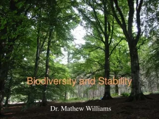
Biodiversity and Stability Dr. Mathew Williams
Complexity and stability • Does a cellular process need all those processes? • Must an organism have so many genes? • Does an ecosystem need all those species? • Are more diverse (complex) ecosystems more or less stable?
Forms of stability • Resilience describes the speed with which a community returns to its former state after perturbation • Resistance describes the ability of a community to avoid displacement in the first place
Resistance and Resilience to Change • Subsistence farmers plant diverse crops to decrease chance of crop failure • Diversity may reduce pest outbreak risks by diluting host availability • Microbial microcosms show less variability in communities with greater species richness (Naeem & Li, 1997)
Resistance to Invasions • Theoretical models suggest that species-poor communities have more empty niches and so are more vulnerable to invasion • Studies of intact ecosystems show both –ve and +ve correlations between species richness and invasion • Vulnerability is probably strongly governed by traits of resident and invading species rather than species richness per se • Absence of parasites is often critical for invasive success
History of the biodiversity-stability debate • Early ideas of Elton and MacArthur • The models of May and others • Combinatorial biodiversity experiments • New approaches to modelling
MacArthur’s ideas (1955) • If a population has diverse predator and prey species, then… • Changes in overall population abundance are buffered against declines in the density of individual species • Insurance hypothesis: more diverse communities can express a greater range of responses to environmental perturbation
Elton’s observation • “simple communities are… more easily upset… than richer ones, that is, more subject to destructive oscillations in populations and more vulnerable to invasions” (Elton, 1958)
Elton’s arguments • Models of 2 interacting species are unstable • Lab communities of 2 or few species are difficult to maintain • Islands (species-poor) are more vulnerable to invasions than continents • Crop monocultures are vulnerable to pests • Species-rich tropical forests are less noted for insect outbreaks than boreal forests
Counter arguments • May has disproved the modelling assumption • Multi-species lab communities crash (BIOSPHERE II) • Introduced species can become pests on continents • Natural monocultures (salt marsh, bracken) seem stable • Insect abundance does fluctuate markedly in tropical forests
May’s Model (1973) • Created randomly constructed simulated communities with randomly assigned interaction strengths • “we consider a simple mathematical model for a many-predator-many-prey system, and show it to be in general less stable, and never more stable, than the analogous one-predator-one-prey community” • Diversity tended to destabilize community dynamics
May’s Model: interactions bij measures the effect of species j’s density on species i’s rate of increase If bij & bji = 0, then there is no effect bij & bji arenegative for competing species bij positive & bji negative for predator (i) and prey (j)
May’s Model: set up Set all bii = –1 (self-regulatory terms) All other b values randomly assigned b = average ‘interaction strength’ (ignore 0 and sign) S = number of species C = connectance (the fraction of all possible pairs of species that interacted directly)
May’s Model: Results Food webs are only likely to be stable if: species, connectance, interaction strength instability b(SC)<1
Model versus Nature • "the balance of evidence would seem to suggest that, in the real world, increased complexity is usually associated with greater stability. There is no paradox here....The real world is no general system. Nature represents a small and special part of parameter space [shaped ultimately by evolutionary forces acting on individuals]“ (May)
Interpretation • real ecosystems "develop" by adding, and losing, species over time, not by randomly sampling ecological possibilities. • But there are no necessary, unavoidable connections linking stability to complexity
Random versus real • Randomly assembled foodwebs can be biologically unreasonable (e.g. loops) • Reasonable foodwebs : • Are more stable than unreasonable ones (studies by Lawlor and by Pimm) • Do not have a sharp transition zone from stability to instability
Bottom-up controls • Bottom-up or donor control: consumer populations are affected by food supply, but not vice versa (bij > 0 , bji = 0) • Stability is unaffected by or increases with complexity (DeAngelis, 1975) • Examples are detritivores, seed-eaters, parasitoid-host systems
Response to Perturbations • Pimm (1979) created 6-species communities (2 predators, 2 intermediate, 2 basal species) • Varied connectance (i.e. complexity) • Removal of top predator stability decreased with increasing complexity • Removal of “basal” species (plants) stability increased with increasing complexity
Is there supporting evidence for May’s model? • If we assume b is constant, then species rich communities (high S) must have less connectance (C) to remain as stable • Field data show that C can increase, fall or stay the same with changes in S b(SC)<1
Experimental Approaches • Combinatorial methods are commonly used to investigate all types of complexity • The process is to deconstruct biological systems into their separate parts… • …and then systematically reconstruct arrays of replicate systems that vary in combinations of parts
Combinatorial biodiversity experiments Complex ecosystem, 8 species (Naeem, 2002)
Biomass (plot size) Varies among replicates Complementarity Sampling effect (Naeem, 2002)
Large reductions in size indicate Little resistance (Naeem, 2002) Fast recovery is indicative of resilience
Diversity-dependent production can decrease stability Pfisterer & Schmid, 2002
Effects of drought perturbation on richness-production relations control drought Ratio between pre- and post-drought 1 year later Pfisterer & Schmid, 2002
Rearranging the insurance hypothesis? • Hypothesis: species-rich systems are more productive because of niche-complementarity • Perturbation disrupts complementarity • Perturbed diverse communities thus suffer more than simple communities lacking complementarity
Conclusions? • Problems with this experiment: • small, short term, does not include other contributors to the food web, such as herbivores or decomposers, looked only at drought • Problems with the conclusions: • sampling could still be an issue • Key output: the relationship between diversity and stability may be determined by pre-stress relationship between diversity and productivity
New approaches to modelling • Use empirical measures of interaction strength • Non-equilibrium dynamics • Food webs consistent with nature • Biomass is the model currency • Consumption rates become saturated as resource density increases
Coupled oscillators • Food chains can be seen as coupled oscillators (e.g a consumer & a resource) • Cyclic dynamics result when oscillators are commensurate • Quasi-periodic or chaotic dynamics result when the oscillators are incommensurate
Corollories • Stabilizing all the underlying oscillators eliminates the occurrence of cyclic or chaotic dynamics in the full system • Reducing the amplitude of the underlying oscillators reduces the amplitude of the dynamics of the full system. • Therefore, inhibiting strong consumer–resource interactions within a food web promotes persistence in food webs.
Three mechanisms inhibit oscillatory subsystems • Apparent competition mechanism (a consumer preys on multiple resources) • Exploitative competition mechanism (two consumers compete for the same resource) • Food-chain-predation mechanism (top predator reduces consumer’s attack rate on resource item)
P = predator C = consumer R = resource a: simple food chain b: exploitative competition c: apparent competition d: intra-guild predation McCann et al (1998)
Exploitative competition C2 can invade once IC2R/IC1R 0.102 Below this value the original food chain (P–C1–R) remains intact and chaotic Once C2 invades, dynamics become simpler Once RIS > 0.15, the system moves towards chaos. The new C2–R interaction has become too strong and no longer dampens the system.
Apparent competition Simple dynamics for RIS <0.12 Above this value C1 or C2 or even P are knocked out Weak links simplify and bound the dynamics
Intra-guild predation We expect the apparent competition mechanism to inhibit the C1–R subsystem and we expect the food-chain mechanism to inhibit the C2–R subsystem. 2 inhibitors and 3 potential oscillators => the dynamics never reach a locally stable equilibrium.
Stable case 1. Set IC2R/IC1R = 0.11 2. Add the apparent competition mechanism 3. P-C1 system inhibited 4. Local stable solution for weak interaction strengths
Testable predictions • Relatively weak interactions coupled to strong interactions reduce oscillations • Food webs with many weak interactions should be less chaotic • Generalist dominated food webs should exhibit less variable dynamics than specialist dominated webs • Depauperate food webs should be more oscillatory than reticulate webs • Data suggest a strong skew towards weak interactions
Random versus actual communities • Compiled food-web relationships with plausible interaction strengths are more stable than randomly constructed food webs • This suggests that interaction strength is critical for stability
What you should have learned today • A history of the biodiversity-stability debate • The utility of combinatorial experiments • The insights that modelling brings to the debate • And that the debate continues.
References • McCann K, Hastings A, Huxel GR (1998) Weak trophic interactions and the balance of nature. Nature, 395, 794-798. • McCann KS (2000) The diversity–stability debate. Nature, 405, 228-233. • Naeem S (2002) Biodiversity equals instability? Nature, 406, 23-24. • Pfisterer AB, Schmid B (2002) Diversity-dependent production can decrease the stability of ecosystem functioning. Nature, 416, 84-86.
Reading from last week • Pfisterer. A.B. & B. Schmid. 2002. Diversity-dependent production can decrease the stability of ecosystem functioning. Nature 416 84-86 • what insights does this experiment provide? • what are the criticisms of the approach? • McCann, K., A. Hastings G. R. Huxel. 1998. Weak trophic interactions and the balance of nature. Nature 395 794-8 • what insights does the modelling provide? • what are the criticisms of the approach?