Implementing Regression Models: Analyzing Beef Consumption and Price Relationships
410 likes | 547 Vues
This presentation outlines the process of implementing a regression model focused on beef consumption in relation to beef prices. It covers essential steps including model fitting, evaluating linear relationships, and assessing goodness-of-fit. The session highlights opportunities for model improvement through exploratory data analysis (EDA) and hypothesis testing. Using real-world data, participants will explore the impact of beef prices on per capita consumption, applying statistical tools to derive insights, interpret results in a business context, and make informed economic assessments.

Implementing Regression Models: Analyzing Beef Consumption and Price Relationships
E N D
Presentation Transcript
Building Demand Models DMD #5 David Kopcso and Richard Cleary BabsonCollege F. W. Olin Graduate School of Business
Agenda • To review the basic steps in implementing a regression model with a specific case study • Fitting the model • Evaluating the strength of the linear relationship • Evaluating the goodness of fit of the model • Forecasting using the model • Evaluating opportunities for improving the model by studying the relationships between the different variables and checking residual assumptions
The Modeling Process • EDA: What relationships do we observe in the sample? • Model: Response Var= b0 + b1 Explanatory Var • Hypothesis: Relationship between variables is linear. • Results: Use StatTools to obtain regression results. • Hypothesis Test • Evaluation (R2 and Standard error of the estimate) • Model interpretation in business/economics setting
Example: Beef Consumption • What are the economic variables you believe influence the demand for beef? • Is there a relationship between Beef consumption per capita and Beef price per pound? • Is this relationship different if substitutes are considered?
The Modeling Process • EDA: What relationships do we observe in the sample? • Model: Beef Consumption PC = b0 + b1 Beef Price • Hypothesis: Relationship between variables is linear. • Results: Use StatTools to obtain regression results. • Hypothesis Test • Evaluation (R2 and Standard error of the estimate) • Model interpretation in business/economics setting
EDA: Correlation Table • StatTools > Summary Stats> Correlations and Covariance
What does CPI tell us? • The data set contains nominal prices, which are unadjusted for inflation. We can adjust for the effects of inflation by converting nominal prices into real prices. In so doing, we can put the values on a “constant ruler”, namely in constant 1982-1984 dollars and cents. This is done as: • Real price = (nominal price/CPI)*100, where CPI is the consumer price index for that year.
Model • Population Model: • Beef Cons PC = 0 + 1 Real Beef Price + ε • Estimated Equation: • Est. Beef Cons PC = b0 + b1 Real Beef Price • •
Hypothesis: No Linear Relationship • 1. Is there is a (linear) relationship between X & Y ? • 2. Hypotheses, stated mathematically: • H0: 1 = 0 (No Linear Relationship) • H1: 1 0 (Linear Relationship) • 3. Compare p-value to a • If p-value is less than or equal to a, then reject null hypothesis, which would indicate there is a linear relationship between Beef Consumption and Beef Price. Business/economic Interpretation - If p-value is less than or equal to a, we would have enough information to conclude that a change in Beef Price would influence a change in Beef Consumption.
Model Interpretation: • b1: The “additional” average amount of beef consumption per capita (in pounds), for every 1 additional cent in (real) beef price per pound. • Beef Consumption decreases by 0.0748 pounds on average for every one additional cent increase in (real) Beef Price per pound. What does the P-value tell us? • b0: The average beef consumption per capita when real beef price per pound equals zero. • Average value of beef consumption per capita is 118.8 pounds when there is no real beef price per pound. • Does this statement make sense? Does this result have managerial/economic significance?
Results: Evaluation • Coefficient of determination (R2) • The closer the R2 to 1, the better the “fit” • R2 is simply the square of the correlation • Standard error of the estimate: S or SEE • The smaller the S, the better the “fit” • The units of S are the same as the units of Y
2 • R Results: R2 • Proportion of variation ‘explained’ by the relationship between X & Y • 3.1% of the variation of beef consumption is explained (determined) by knowing the beef price. • Explained Variance • • Total Variance
Results: Standard Error of Estimate • Measures variation of the observed values from predicted values, i.e., the amount of error one expects when using the regression equation for prediction. • On average, we would expect 68% of actual beef consumption to be within 9.07 pounds of predicted per capita beef consumption. • Within how many pounds of the predicted beef consumption per capita would we expect 95% of beef consumption to be?
What does economic theory say? • Recall: The sign of the coefficient is negative as was expected: it implies that a 1 cent increase in the real price of beef (retail) reduces consumption of beef per capita by 0.075 lbs on average. We noticed that the real price coefficient makes an insignificant contribution to beef consumption (since its p-value is greater than your level of significance, usually 0.05). This is probably because the model has excluded relevant variables.
Consider the following regression model: • Beef Consumption PC = • β0 + β1 * Real Beef Price + β2 * Real Chicken Price + ε
Discuss R2, SEE, and the slopes • R2 tells us that 62% of the variation in Beef consumption is explainable by knowing real beef price and real chicken prices. • SEE, the standard error of the estimate, gives us a rough estimate of how closely the regression equation fits the data. In particular about two-thirds (68%) of the data should fall within +/- 5.7708 lbs. of the value determined by the regression equation. Similarly about 95% of the data fall within 2* 5.7708, or 11.5416 lbs. of the value determined by the regression equation. • The slope coefficient in front of real beef price is -0.1459, which means if real chicken price is held constant, for each additional 1 cent increase in real beef price, beef consumption will decrease 0.1459 lbs on average. Similarly, the slope coefficient for real chicken price is 0.3429, which means that if real beef price is held constant, for each additional 1 cent increase in real chicken price beef consumption will increase 0.3429 lbs on average.
Discuss the constant and p-values • The constant, 102.77 lbs, has no real interpretation here since none of the data values are around real beef and real chicken prices of 0. • Assuming a level of significance of 5%, we see that all the p-values in the output are less than the level of significance, 5%. The p-value from the ANOVA Table has a value of 0.0000 and tells us that there is at least one of the explanatory variables that is useful in this model. The p-value from the Regression coefficients table in the RealBeefPrice row has a value of 0.0039 and tells us that RealBeefPrice, taking into account RealChickenPrice, is useful in this model. Similarly, the p-value from the Regression coefficients table in the RealChickenPrice row has a value of 0.0000 and tells us that RealChickenPrice, taking into account RealBeefPrice, is useful in this model.
Why does this model make sense from an economic point of view? • Compared to the previous model, this model makes sense economically, for it includes another key determinant of demand. The estimated model is: • BeefConsump =102.8 – 0.15* RealBeefPrice + 0.34* RealChickenPrice • The signs are in agreement with economic theory. Chicken is a substitute for beef, and therefore the coefficient of its price should be positive. The R2 of this regression is 0.62, a vast improvement over the R2 of the previous regression, 0.03. Notice also how the coefficient on real price of beef (retail) has changed dramatically compared to the previous regression.
Include/Exclude Decision • When refining models, drop the variable with the highest p-value above the significance level first. • Drop only one variable at a time. The values will change upon re-estimating the model. • Do not drop any ‘confirmatory’ variables.
Questions • Is DPI a confirmatory variable in today’s Beef Consumption Model? We’ll see in Microeconomics (Mod II) that it is. • Examine the residual plots of the full Beef Consumption Model. • Is the number of Bathrooms a confirmatory variable in the House Price example from DMD 04? • What is the expectation of the number of bathrooms in a house today? What was it in 1950?
Further issues • Although the last Beef Consumption model is sufficient, and clearly more informative than ignoring the relationships, we are left with a few nagging concerns. • The R2 shows that we still have 38% of the variation in beef consumption left unexplained. • The graphs or scatterplots do not exhibit linear relationships. • Real DPI is insignificant, i.e., p-value > a. So we can’t interpret its coefficient..
What Next? We next turn to the residuals. Perhaps some insights are available by investigating the residuals.
Residuals • A residual is the numerical value of the difference between the actual value and the predicted value. There is one residual value for each data value. • The main purpose of residuals is to check the assumptions of a regression analysis.
Catch 22 • We cannot check the regression requirements (assumptions) until after running the regression analysis. • This does not mean we can choose to ignore the assumptions. Often, insights into the relationships are found via a residual analysis.
Linear Regression Assumptions Residual Analysis 1. Normality Probability distribution (histogram) of residuals is Normal. 2. Constant Variance Scatterplot of residuals vs. each X variable appears random. First inspect the scatterplot of residuals vs. the fitted values 3. Linearity Scatterplot of Y vs. each X suggests linear relationship. Again, first inspect the scatterplot of residuals vs. the fitted values
Is the relationship between the Residuals and Real DPI linear?
Is the relationship between the Residuals and Real DPI quadratic?
Transforming to Linear • Clearly, the graphs of the data and of the residuals show a curved pattern indicating that the relationship is non linear. The vertex of this parabola is approximately at $11061 which is the mean of RDPI. • By transforming the data, we can create a linear pattern. For example, if the relationship appears quadratic, then we square the data and run the following model: Y = β0 + β1* X + β2* X2 + ε
Transforming to Linear • Since the vertex of this parabola is approximately at RDPI = $11061, which is the mean of RDPI, we will use the following transformation: • Instead of using the RDPI variable as our indicator of income we will use the variable (RDPI-11061)^2. • Let’s see if this new variable is significant and if there is a real economic interpretation of this transformation.
Does this transformed variable seem linearly related to Beef Consumption?
Regression Results of Transformed Model:
Linear Regression Assumptions:Residual Analysis 1. Normality Probability distribution (histogram) of residuals is Normal. 2. Constant Variance Scatterplot of residuals vs. each X variable appears random. First inspect the scatterplot of residuals vs. the fitted values 3. Linearity Scatterplot of Y vs. each X suggests linear relationship. Again, first inspect the scatterplot of residuals vs. the fitted values