### Neural Network Time Representation for Stock Prediction and Motion Detection ###
This lecture explores the design and application of neural networks for tasks involving time representation, such as predicting stock prices and detecting motion in surveillance systems. For stock prediction, the input consists of normalized past values to train a backpropagation network for future price estimation. For motion detection, two successive images are concatenated to create a comprehensive input vector. The lecture emphasizes the importance of exemplar analysis, ensuring coverage of the problem space, and the need to train networks on both classifiable and "garbage" data for better classification accuracy. ###

### Neural Network Time Representation for Stock Prediction and Motion Detection ###
E N D
Presentation Transcript
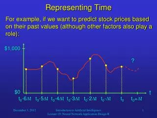
$1,000 ? t0-6t t0-5t t0-4t t0-3t t0-2t t0-t t0 t0+t Representing Time • For example, if we want to predict stock prices based on their past values (although other factors also play a role): $0 t Introduction to Artificial Intelligence Lecture 19: Neural Network Application Design II
Representing Time • In this case, our input vector would include seven components, each of them indicating the stock values at a particular point in time. • These stock values have to be normalized, i.e., divided by $1,000, if that is the estimated maximum value that could occur. • Then there would be a hidden layer, which usually contains more neurons than there are input neurons. • And there could be exactly one output neuron, indicating the stock price after the following time interval (to be multiplied by $1,000). Introduction to Artificial Intelligence Lecture 19: Neural Network Application Design II
Representing Time • For example, a backpropagation network could do this task. • It would be trained with many stock price samples that were recorded in the past so that the price for time t0 + t is already known. • This price at time t0 + t would be the desired output value of the network and be used to apply the BPN learning rule. • Afterwards, if past stock prices indeed allow the prediction of future ones, the network will be able to give some reasonable stock price predictions. Introduction to Artificial Intelligence Lecture 19: Neural Network Application Design II
Representing Time • Another example: • Let us assume that we want to build a very simple surveillance system. • We receive bitmap images in constant time intervals and want to determine for each quadrant of the image if there is any motion visible in it, and what the direction of this motion is. • Let us assume that each image consists of 10 by 10 grayscale pixels with values from 0 to 255. • Let us further assume that we only want to determine one of the four directions N, E, S, and W. Introduction to Artificial Intelligence Lecture 19: Neural Network Application Design II
Representing Time • As said before, it makes sense to represent the brightness of each pixel by an individual analog value. • We normalize these values by dividing them by 255. • Consequently, if we were only interested in individual images, we would feed the network with input vectors of size 100. • Let us assume that two successive images are sufficient to detect motion. • Then at each point in time, we would like to feed the network with the current image and the previous image that we received from the camera. Introduction to Artificial Intelligence Lecture 19: Neural Network Application Design II
Representing Time • We can simply concatenate the vectors representing these two images, resulting in a 200-dimensional input vector. • Therefore, our network would have 200 input neurons, and, as usual, 200 or more hidden units. • With regard to the output, would it be a good idea to represent the direction (N, E, S, or W) by a single analog value? • No, these values do not represent a scale, so this would make the network computations unnecessarily complicated. Introduction to Artificial Intelligence Lecture 19: Neural Network Application Design II
Representing Time • Better solution: • 16 output neurons with the following interpretation: This way, the network can, in a straightforward way, indicate the direction of motion in each quadrant (Q1, Q2, Q3, and Q4). Each output value could specify the amount (or speed?) of the corresponding type of motion. Introduction to Artificial Intelligence Lecture 19: Neural Network Application Design II
Exemplar Analysis • When building a neural network application, we must make sure that we choose an appropriate set of exemplars (training data): • The entire problem space must be covered. • There must be no inconsistencies (contradictions) in the data. • We must be able to correct such problems without compromising the effectiveness of the network. Introduction to Artificial Intelligence Lecture 19: Neural Network Application Design II
Ensuring Coverage • For many applications, we do not just want our network to classify any kind of possible input. • Instead, we want our network to recognize whether an input belongs to any of the given classes or it is “garbage” that cannot be classified. • To achieve this, we train our network with both “classifiable” and “garbage” data (null patterns). • For the the null patterns, the network is supposed to produce a zero output, or a designated “null neuron” is activated. Introduction to Artificial Intelligence Lecture 19: Neural Network Application Design II
Ensuring Coverage • In many cases, we use a 1:1 ratio for this training, that is, we use as many null patterns as there are actual data samples. • We have to make sure that all of these exemplars taken together cover the entire input space. • If it is certain that the network will never be presented with “garbage” data, then we do not need to use null patterns for training. Introduction to Artificial Intelligence Lecture 19: Neural Network Application Design II
Ensuring Consistency • Sometimes there may be conflicting exemplars in our training set. • A conflict occurs when two or more identical input patterns are associated with different outputs. • Why is this problematic? Introduction to Artificial Intelligence Lecture 19: Neural Network Application Design II
Ensuring Consistency • Assume a BPN with a training set including the exemplars (a, b) and (a, c). • Whenever the exemplar (a, b) is chosen, the network adjust its weights to present an output for a that is closer to b. • Whenever (a, c) is chosen, the network changes its weights for an output closer to c, thereby “unlearning” the adaptation for (a, b). • In the end, the network will associate input a with an output that is “between” b and c, but is neither exactly b or c, so the network error caused by these exemplars will not decrease. • For many applications, this is undesirable. Introduction to Artificial Intelligence Lecture 19: Neural Network Application Design II
Ensuring Consistency • To identify such conflicts, we can apply a (binary) search algorithm to our set of exemplars. • How can we resolve an identified conflict? • Of course, the easiest way is to eliminate the conflicting exemplars from the training set. • However, this reduces the amount of training data that is given to the network. • Eliminating exemplars is the best way to go if it is found that these exemplars represent invalid data, for example, inaccurate measurements. • In general, however, other methods of conflict resolution are preferable. Introduction to Artificial Intelligence Lecture 19: Neural Network Application Design II
Ensuring Consistency • Another method combines the conflicting patterns. • For example, if we have exemplars • (0011, 0101),(0011, 0010), • we can replace them with the following single exemplar: • (0011, 0111). • The way we compute the output vector of the new exemplar based on the two original output vectors depends on the current task. • It should be the value that is most “similar” (in terms of the external interpretation) to the original two values. Introduction to Artificial Intelligence Lecture 19: Neural Network Application Design II
Ensuring Consistency • Alternatively, we can alter the representation scheme. • Let us assume that the conflicting measurements were taken at different times or places. • In that case, we can just expandall the input vectors, and the additional values specify the time or place of measurement. • For example, the exemplars • (0011, 0101),(0011, 0010) • could be replaced by the following ones: • (100011, 0101),(010011, 0010). Introduction to Artificial Intelligence Lecture 19: Neural Network Application Design II
Ensuring Consistency • One advantage of altering the representation scheme is that this method cannot create any new conflicts. • Expanding the input vectors cannot make two or more of them identical if they were not identical before. Introduction to Artificial Intelligence Lecture 19: Neural Network Application Design II
Training and Performance Evaluation • When training a BPN, what is the acceptable error, i.e., when do we stop the training? • The minimum error that can be achieved does not only depend on the network parameters, but also on the specific training set. • Thus, for some applications the minimum error will be higher than for others. • As a rule of thumb, any BPN should always be able to reach an error of 0.2 or better. Introduction to Artificial Intelligence Lecture 19: Neural Network Application Design II
Training and Performance Evaluation • A more insightful way of performance evaluation is partial-set training. • The idea is to split the available data into two sets – the training set and the test set. • The network’s performance on the second set indicates how well the network has actually learned the desired mapping. • We should expect the network to interpolate, but not extrapolate. • Therefore, this test also evaluates our choice of training samples. Introduction to Artificial Intelligence Lecture 19: Neural Network Application Design II
Training and Performance Evaluation • If the test set only contains one exemplar, this type of training is called “hold-one-out” training. • It is to be performed sequentially for every individual exemplar. • This, of course, is a very time-consuming process. Introduction to Artificial Intelligence Lecture 19: Neural Network Application Design II
Example I: Predicting the Weather • Let us study an interesting neural network application. • Its purpose is to predict the local weather based on a set of current weather data: • temperature (degrees Celsius) • atmospheric pressure (inches of mercury) • relative humidity (percentage of saturation) • wind speed (kilometers per hour) • wind direction (N, NE, E, SE, S, SW, W, or NW) • cloud cover (0 = clear … 9 = total overcast) • weather condition (rain, hail, thunderstorm, …) Introduction to Artificial Intelligence Lecture 19: Neural Network Application Design II
100 km Example I: Predicting the Weather • We assume that we have access to the same data from several surrounding weather stations. • There are eight such stations that surround our position in the following way: Introduction to Artificial Intelligence Lecture 19: Neural Network Application Design II
Example I: Predicting the Weather • Which network type is most suitable for this kind of application? • The network is supposed to produce a mapping from the current weather conditions to the predicted conditions for the next day. • Both the BPN and the CPN could do this task. • However, the BPN is better at generalizing, that is, yielding plausible outputs for untrained inputs. • Therefore, we decide to use a BPN for our weather application. Introduction to Artificial Intelligence Lecture 19: Neural Network Application Design II
Example I: Predicting the Weather • How should we format the input patterns? • We need to represent the current weather conditions by an input vector whose elements range in magnitude between zero and one. • When we inspect the raw data, we find that there are two types of data that we have to account for: • Scaled, continuously variable values • n-ary representations of category values Introduction to Artificial Intelligence Lecture 19: Neural Network Application Design II
Example I: Predicting the Weather • The following data can be scaled: • temperature (-10… 40 degrees Celsius) • atmospheric pressure (26… 34 inches of mercury) • relative humidity (0… 100 percent) • wind speed (0… 250 km/h) • cloud cover (0… 9) • We can just scale each of these values so that its lower limit is mapped to 0 and its upper value is mapped to 1. • These numbers will be the components of the input vector. Introduction to Artificial Intelligence Lecture 19: Neural Network Application Design II
Example I: Predicting the Weather • Usually, wind speeds vary between 0 and 40 km/h. • By scaling wind speed between 0 and 250 km/h, we can account for all possible wind speeds, but usually only make use of a small fraction of the scale. • Therefore, only the most extreme wind speeds will exert a substantial effect on the weather prediction. • Consequently, we will use two scaled input values: • wind speed ranging from 0 to 40 km/h • wind speed ranging from 40 to 250 km/h Introduction to Artificial Intelligence Lecture 19: Neural Network Application Design II
Example I: Predicting the Weather • How about the non-scalable weather data? • Wind direction is represented by an eight- component vector, where only one element (or possibly two adjacent ones) is active, indicating one out of eight wind directions. • The subjective weather condition is represented by a nine-component vector with at least one, and possibly more, active elements. • With this scheme, we can encode the current conditions at a given weather station with 23 vector components: • one for each of the four scaled parameters • two for wind speed • eight for wind direction • nine for the subjective weather condition Introduction to Artificial Intelligence Lecture 19: Neural Network Application Design II
… … … our station north northwest Example I: Predicting the Weather • Since the input does not only include our station, but also the eight surrounding ones, the input layer of the network looks like this: … The network has 207 input neurons, which accept 207-component input vectors. Introduction to Artificial Intelligence Lecture 19: Neural Network Application Design II