Data preparation: Selection, Preprocessing, and Transformation
Data preparation: Selection, Preprocessing, and Transformation. Literature: I.H. Witten and E. Frank, Data Mining, chapter 2 and chapter 7. Knowledge. Transformed data. Patterns. Target data. Processed data. Interpretation Evaluation. Data Mining. Transformation & feature


Data preparation: Selection, Preprocessing, and Transformation
E N D
Presentation Transcript
Data preparation: Selection, Preprocessing, and Transformation • Literature: • I.H. Witten and E. Frank, Data Mining, chapter 2 and chapter 7
Knowledge Transformed data Patterns Target data Processed data Interpretation Evaluation Data Mining Transformation & feature selection Preprocessing & cleaning Selection Fayyad’s KDD Methodology data
Contents • Data Selection • Data Preprocessing • Data Transformation
Data Selection • Goal • Understanding the data • Explore the data: • possible attributes • their values • distribution, outliers
Getting to know the data • Simple visualization tools are very useful for identifying problems • Nominal attributes: histograms (Distribution consistent with background knowledge?) • Numeric attributes: graphs (Any obvious outliers?) • 2-D and 3-D visualizations show dependencies • Domain experts need to be consulted • Too much data to inspect? Take a sample!
Data preprocessing • Problem: different data sources (e.g. sales department, customer billing department, …) • Differences: styles of record keeping, conventions, time periods, data aggregation, primary keys, errors • Data must be assembled, integrated, cleaned up • “Data warehouse”: consistent point of access • External data may be required (“overlay data”) • Critical: type and level of data aggregation
Data Preprocessing • Choose data structure (table, tree or set of tables) • Choose attributes with enough information • Decide on a first representation of the attributes (numeric or nominal) • Decide on missing values • Decide on inaccurate data (cleansing)
Attribute types used in practice • Most schemes accommodate just two levels of measurement: nominal and ordinal • Nominal attributes are also called “categorical”, “enumerated”, or “discrete” • But: “enumerated” and “discrete” imply order • Special case: dichotomy (“boolean” attribute) • Ordinal attributes are called “numeric”, or “continuous” • But: “continuous” implies mathematical continuity
The ARFF format % ARFF file for weather data with some numeric features % @relation weather @attribute outlook {sunny, overcast, rainy} @attribute temperature numeric @attribute humidity numeric @attribute windy {true, false} @attribute play? {yes, no} @data sunny, 85, 85, false, no sunny, 80, 90, true, no overcast, 83, 86, false, yes ...
Attribute types • ARFF supports numeric and nominal attributes • Interpretation depends on learning scheme • Numeric attributes are interpreted as • ordinal scales if less-than and greater-than are used • ratio scales if distance calculations are performed • (normalization/standardization may be required) • Instance-based schemes define distance between nominal values (0 if values are equal, 1 otherwise) • Integers: nominal, ordinal, or ratio scale?
Nominal vs. ordinal • Attribute “age” nominalIf age = young and astigmatic = no and tear production rate = normal then recommendation = softIf age = pre-presbyopic and astigmatic = no and tear production rate = normal then recommendation = soft • Attribute “age” ordinal(e.g. “young” < “pre-presbyopic” < “presbyopic”)If age pre-presbyopic and astigmatic = no and tear production rate = normal then recommendation = soft
Missing values • Frequently indicated by out-of-range entries • Types: unknown, unrecorded, irrelevant • Reasons: malfunctioning equipment, changes in experimental design, collation of different datasets, measurement not possible • Missing value may have significance in itself (e.g. missing test in a medical examination) • Most schemes assume that is not the case “missing” may need to be coded as additional value
Inaccurate values • Reason: data has not been collected for mining it • Result: errors and omissions that don’t affect original purpose of data (e.g. age of customer) • Typographical errors in nominal attributes values need to be checked for consistency • Typographical and measurement errors in numeric attributes outliers need to be identified • Errors may be deliberate (e.g. wrong zip codes) • Other problems: duplicates, stale data
TransformationAttribute selection • Adding a random (i.e. irrelevant) attribute can significantly degrade C4.5’s performance • Problem: attribute selection based on smaller and smaller amounts of data • IBL is also very susceptible to irrelevant attributes • Number of training instances required increases exponentially with number of irrelevant attributes • Naïve Bayes doesn’t have this problem. • Relevant attributes can also be harmful
Scheme-independent selection • Filter approach: assessment based on general characteristics of the data • One method: find subset of attributes that is enough to separate all the instances • Another method: use different learning scheme (e.g. C4.5, 1R) to select attributes • IBL-based attribute weighting techniques can also be used (but can’t find redundant attributes) • CFS: uses correlation-based evaluation of subsets
Searching the attribute space • Number of possible attribute subsets is exponential in the number of attributes • Common greedy approaches: forward selection and backward elimination • More sophisticated strategies: • Bidirectional search • Best-first search: can find the optimum solution • Beam search: approximation to best-first search • Genetic algorithms
Scheme-specific selection • Wrapper approach: attribute selection implemented as wrapper around learning scheme • Evaluation criterion: cross-validation performance • Time consuming: adds factor k2 even for greedy approaches with k attributes • Linearity in k requires prior ranking of attributes • Scheme-specific attribute selection essential for learning decision tables • Can be done efficiently for DTs and Naïve Bayes
Discretizing numeric attributes • Can be used to avoid making normality assumption in Naïve Bayes and Clustering • Simple discretization scheme is used in 1R • C4.5 performs local discretization • Global discretization can be advantageous because it’s based on more data • Learner can be applied to discretized attribute or • It can be applied to binary attributes coding the cut points in the discretized attribute
Unsupervised discretization • Unsupervised discretization generates intervals without looking at class labels • Only possible way when clustering • Two main strategies: • Equal-interval binning • Equal-frequency binning (also called histogram equalization) • Inferior to supervised schemes in classification tasks
Entropy-based discretization • Supervised method that builds a decision tree with pre-pruning on the attribute being discretized • Entropy used as splitting criterion • MDLP used as stopping criterion • State-of-the-art discretization method • Application of MDLP: • “Theory” is the splitting point (log2[N-1] bits) plus class distribution in each subset • DL before/after adding splitting point is compared
Formula for MDLP • N instances and • k classes and entropy E in original set • k1 classes and entropy E1 in first subset • k2 classes and entropy E2 in first subset • Doesn’t result in any discretization intervals for the temperature attribute
Other discretization methods • Top-down procedure can be replaced by bottomup method • MDLP can be replaced by chi-squared test • Dynamic programming can be used to find optimum k-way split for given additive criterion • Requires time quadratic in number of instances if entropy is used as criterion • Can be done in linear time if error rate is used as evaluation criterion
Transformation • WEKA provides a lot of filters that can help you transforming and selecting your attributes! • Use them to build a promising model for the caravan data!