
Laplace Transform: Application in Differential Equations
E N D
Presentation Transcript
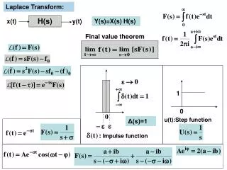
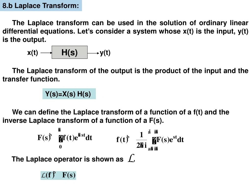
8.b Laplace Transform: H(s) x(t) y(t) The Laplace transform can be used in the solution of ordinary linear differential equations. Let’s consider a system whose x(t) is the input, y(t) is the output. The Laplace transform of the output is the product of the input and the transfer function. Y(s)=X(s) H(s) We can define the Laplace transform of a function of a f(t) and the inverse Laplace transform of a function of a F(s). The Laplace operator is shown as
Final value theorem teoremi: The Laplace transforms of derivatives are given as The transforms of higher order derivatives can be written as well. Final Value Theorem: When t goes to infinity, the value of the limit can be calculated from the Laplace transform. For Exponential/Harmonic functions, when the value of their limit is arrived, it is called as the time at which the steady state value is achieved.
Δ(s)=1 1 u(t):Step function 0 Impulse function Laplace Transform of Impulse and Step Functions: The Laplace transform of the impulse and step functions dependent on t is given in Table. Impulse function is a brief pulse called an approximation of an impulse. Step function is a change from zero to one in a very short time.
Inverse Laplace Transfom: If the eigenvalue is real, the inverse Laplace transform gives as Inverse Laplace Transform If the eigenvalues are complex, the inverse Laplace transform gives as Inverse Laplace Transform
Impulse Response: (Example (8.1) continued) If the input is impulse, its Laplace transform equals to 1. The Laplace transform of the output equals to transfer function itself. Taking the inverse Laplace transform, we can find the impulse response. Here, h(t) is the impulse response. : Inverse Laplace Transform of H(s) Let’s find the impulse response for Example 8.1. In order to find the inverse Laplace transform, we should apply the partial fraction expansion to the transfer function. Remember that, we can find the eigenvalues as below. a=[1,4,14,20];roots(a) Eigenvalues: -1±3i, -2
If the eigenvalues of the system are found, we can write the expression as below. In the process of the partial fraction expansion, denumerators contain eigenvalues while numerators contain the constants to find the response. If eigenvalues are in a complex form, constants in the numerators are in the complex form. The Partial fraction expansion means that the fraction is expressed as a sum of a polynomial and several fractions with a simpler denominator. We can find the portions with the command “residue” in MATLAB program. p1 is the numerator of the transfer function. p2 is the denumerator of the transfer function. p1=[1,3]; p2=[1,4,14,20]; [r,p,k]=residue(p1,p2)
Partial fraction expansion: The command of “residue” gives the results assigning the variables, r, p, and k. The constants are assigned to the variable of r. The eigenvalues are assigned to the variable of p. The variable of k is zero because the order of polinom in the denumerator is higher than the order of polinom in the numerator. The values of r are found as r(1)=-0.05-0.1833i, r(2)=-0.05+0.1833i, r(3)=0.1 The form of the partial fraction expansion of the transfer function is
By using the preceding Table, we can find the inverse Laplace transforms of H(s). The inverse Laplace transform of the first two terms is in the form of Ae-tcos(3t-φ) and Aeiφ=2(-0.05+0.1833i). We can find A and φ by MATLAB commands as follow. z=2*(-0.05+0.1833i ) a=abs(z);fi=angle(z) A and φ are found as a=0.3801 ve φ=1.837. The inverse Laplace transform of the last term is in the form of 0.1e-2t. We can write the impulse response of h(t) as
From the eigenvalues of the system, the damping ratio, time increment and steady-state time, and can be calculated as ξ=0.3162 (s=-1±3i) Δt=0.099, t∞=6.283. Impulse response of the system is plotted by MATLAB program. clc;clear; t=0:0.099:6.283; yt=0.3801*exp(-t).*cos(3*t-1.837)+0.1*exp(-2*t) plot(t,yt) Impulse response is the time behaviour of the output of a general system when its inputs change suddenly in a very short time.
Step Response: Let’s find the unit step response for Example 8.1. The Laplace transform of the output equals the product of 1/s and transfer function. y(t) : Inverse Laplace Transform of Y(s) Eigenvalues : -1±3i , -2 We can find the step response y(t) by taking the inverse Laplace transform of Y(s). By process of the partial fraction expansion, Y(s) is written as
We can write a MATLAB program to find the fractions. The program gives the results as p1=[1,3]; p2=[1,4,14,20,0]; [r,p,k]=residue(p1,p2) r(1)=-0.05+0.0333i, r(2)=-0.05-.0033i, r(3)=-0.05, r(4)=0.15 Y(s) is written in the form of the partial fraction expansion. The inverse Laplace transform of the first two terms is in the form of Ae-tcos(3t-φ) and Aeiφ=2(-0.05-0.03333i). Then, we can write the unit step response of y(t) as
Final value theorem: yss=0.15 Step response of the system is plotted by MATLAB program. clc;clear; t=0:0.099:6.283; yt=0.1202*exp(-t).*cos(3*t+2.5536)-0.05*exp(-2*t)+0.15; plot(t,yt) Step response is the time behaviour of the outputs of a general system when its inputs change from zero to one in a very short time.