
EOFs and PCAs
EOFs and PCAs. Time-Series Analysis. Harmonic Analysis Fourier Expansion Fast Fourier Transform (FFT) Wavelets Empirical Mode Decomposition (EMD) Hilbert-Huang Transform (HHT). The Problem. Multiple time-series of same parameters from different locations (maps>2)

EOFs and PCAs
E N D
Presentation Transcript
Time-Series Analysis • Harmonic Analysis • Fourier Expansion • Fast Fourier Transform (FFT) • Wavelets • Empirical Mode Decomposition (EMD) • Hilbert-Huang Transform (HHT)
The Problem • Multiple time-series of same parameters from different locations (maps>2) • Multiple time-series of different parameters (>2) from the same location. A Manual for EOF and SVD analyses of Climatic Data H. Bjornsson & S. A. Venegas McGill University, 1997
Introduction • “The central idea of principal component analysis (PCA or EOF) is to reduce the dimensionality of a data set consisting of a large number of interrelated variables, while retaining as much as possible of the variation present in the data set. • This is achieved by transforming to a new set of variables, the principle components (or EOFs), which are uncorrelated, and which are ordered so that the first few retain most of the variation present in all of the original variables.” • Jolliffe (2002, p 1).
Empirical Orthogonal Function technique aims at finding a new set of variables (Principal Components, PCs) that capture most of the observed variance from the data through a linear combination of the original variables
EOF Analysis • Data matrix, X(i,j), represents i samples of j variables (mean for each variable has been removed). • xij with i=1,…n (sample no) and j=1,…p (variable)
X1 X2 10.0000 10.7000 10.4000 9.8000 9.7000 10.0000 9.7000 10.1000 11.7000 11.5000 11.0000 10.8000 8.7000 8.8000 9.5000 9.3000 10.1000 9.4000 9.6000 9.6000 10.5000 10.4000 9.2000 9.0000 11.3000 11.6000 10.1000 9.8000 8.5000 9.2000 >> corrcoef(x1,x2) ans = 1.0000 0.8871 0.8871 1.0000 >> cov(x1,x2) ans = 0.7986 0.6793 0.6793 0.7343 >>mean([x1 x2]) ans = 10 10
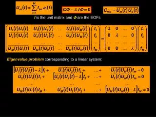
Covariance matrix(Cm,m) of Xn,m The aim of EOF/PCA is to find the linear combination of all the variables, i.e. grid points, that explains maximum variance. That is to find a direction α= (α1, . . . , αp)Tsuch that X α has maximum variability. Now the variance of the (centered) time seriesX∙αis we normally require the vector a to be unitary. Hence the problem readily yields:
The solution is an eigenvalue problem: • Where α is the eigenvector and λ is the eigenvalue. • The kth EOF is the kth eigenvector of ak of C after the eigenvalues and corresponding eigenvectors have been sorted in decreasing order. • The eigenvalueλk corresponding to the kth EOF gives a measure of the explained variance by αk, k=1…p. The explained valiance is written in terms of % as: [V,D] = eig(X) produces a diagonal matrix D of eigenvalues and a full matrix V whose columns are the corresponding eigenvectors so that X*V = V*D.
Principal Component • The projection of the anomaly field X onto the kthEOF ak, i.e., ck = X∙αkis the kthprincipal component (PC):
% [m,k]=size(x); for i=1:k xm(:,i)=x(:,i)-mean(x(:,i)); end % C = cov(xm); [alpha,lambda]=eig(C); Eigenvalue = diag(lambda); [Eigval, Ie] = sort(Eigenvalue,'descend'); Eigenvector = alpha(:,Ie); for i=1:k ypca(:,i)=Eigenvector(:,i)'*xm'; ypca(:,i)=ypca(:,i)+mean(x(:,i)); end
pca1 pca2 9.5169 9.4935 9.8486 10.4208 10.2171 9.7929 10.1481 9.7206 7.7345 10.0879 8.7242 10.1113 11.7689 9.9711 10.8449 10.1614 10.3418 10.5032 10.5655 10.0134 9.3621 10.0556 11.2691 10.1715 7.9550 9.7395 10.0657 10.2137 11.6376 9.5436 X1 X2 10.0000 10.7000 10.4000 9.8000 9.7000 10.0000 9.7000 10.1000 11.7000 11.5000 11.0000 10.8000 8.7000 8.8000 9.5000 9.3000 10.1000 9.4000 9.6000 9.6000 10.5000 10.4000 9.2000 9.0000 11.3000 11.6000 10.1000 9.8000 8.5000 9.2000 >> cov(x1,x2) ans = 0.7986 0.6793 0.6793 0.7343 >> corrcoef(x1,x2) ans = 1.0000 0.8871 0.8871 1.0000 >>mean([x1 x2]) ans= 10 10 >>cov(ypca) ans = 1.4465 0.0000 0.0000 0.0864 >> corrcoef(ypca) ans = 1.0000 0.0000 0.0000 1.0000 >>mean(ypca) ans= 10.0000 10.0000
EOF of a Single Field/Parameter • Assume we have p (maps) of time series with a length n each F(n,p) • Remove the mean from each column (centered values) • Form the covariance matrix R=FT·F • Solve the Eigenvalue problem R∙C=C·Λ (see MATLAB® function eig.m) • Λ is a diagonal matrix containing the eigenvaluesλi of R. • The ci column vectors of C are the eigenvectors of R corresponding to the eigenvaluesλi. Both Λ and C have size p x p • For each eigenvalue (λi ) we find the corresponding eigenvector ci. Each eigenvector can be regarded as a map. These are the EOFs. • Order eigenvectors according to the size of the eigenvalue (descending order). • EOF1 is the eigenvector associated with the biggest eigenvalue, EOF2 the one associated with the 2nd largest etc. • Each eigenvalueλi gives a measure of the amount of total variance R explained by that eigenvector ci. The fraction is found by dividing λi by the trace of Λ.
In MATLAB® function [PC,eof,DSUM,Z]=EOF_gv(F) Z=detrend(F,0); % you might also normalize by dividing by the std of each column S=Z'*Z; % Covariance Matrix (cov(Z) or S=1/(n-1)S, where n no of columns) [E,d]=eig(cov(Z)); % Solve eigenvector problem X*V = V*D; E eigenvectors in columns &d is the eigenvalues dsum=100*diag(d)/trace(d); % d/sum(d) in percent [DSUM,I]=sort(dsum,'descend'); % Sort Eigenvalues in terms of importance, 1 the most important eof=E(:,I); % Re-arrange eigenvectors according to their eigenvalues PC =Z*eof ; % Principal component terms- expansion coefficients -amplitudes Nn=3; % select number of EOFs to be used (example in here is 3) Z=PC(:,Nn)*eof(:,Nn)‘; % Recreate the original matrix using reduced EOFS Zo=PC*eof‘; % Recreate the original matrix using all EOFS end % if Zo is not almost identical to F then check your method
Exercise • Create a function that can perform EOF/PCA to a matrix of data. • Rotate the velocity data (u,v) using PCA. • Rotate the velocity data (u,v,w) using PCA
EOF History • Lorenz (1956) invented empirical orthogonal functions (EOFs) because he saw that they could be of use in statistical forecasting; EOFs were also invented, independently, by statisticians. • Lorenz never published his EOF study in a journal. The goal of his study was to find a way to extract a compact or simplified but “optimal” representation of data with both space and time dependence, e.g., a time sequence of sea-level pressure maps. His approach was to expand the data in terms of optimally defined functions of space, each of which is associated with a time-dependent “amplitude.” Lorenz, E. N., 1956: Empirical orthogonal functions and statistical weather prediction. Sci. Rep. No. 1, Statistical Forecasting Project, M.I.T., Cambridge, MA, 48 pp.
The pattern obtained when an EOF is plotted as a map represents a standing oscillation. • The time-evolution of an EOF is expressed through the amplitude (αi) of the standing oscillation changing over time and is estimated as: • We can reconstruct the data from the EOFs and the expansion coefficients:
Example (Beach Profiles) function [t,x,Y]=beach % x = [1:120]; t = [0:0.5:23.5]; n = length(t); y = exp(-0.03*x); z1 =zeros(size(x)); zb=0.4*sin(2*pi*[0:50]/50); z1(40:90)=zb; % for i=1:n f1=cos(2*pi*t(i)/8); f2=cos(2*pi*t(i)/8+pi); Y(:,i)=y+z1*f1; end t=23.5mo t=0 for i=1:48; plot(x,Y(:,i)+(i-1)*0.10); hold on; end
The Matrix ///-///-///-///-/// Coastline ///-///-///-///-/// + - - + >> [PC,eof,DSUM,Z]=EOF_gv(Y)
EOF Analysis • [t,X,Y]=beach • [A,eof,DSUM,Z]=EOF_gv(Y) • plot([1:length(DSUM)],DSUM) • plot(t, eof(:,1), t, eof(:,2), t, eof3(:,3)) • plot(X,A(:,1),X,A(:,2),X,A(:,3))
Errors in EOF • Rule of thumb (North et al., 1982) • Error in eigenvalueλ: • Error in expansion (eigenfactor) coefficient: where λj is the closest eigenvalue to λk • Monte Carlo Simulations North, G. R., T. L., Bell, R. F. Cahalan, and F. J. Moeng, 1982: Sampling errors in the estimation of empirical orthogonal functions. Mon. Weather Rev., 110, 699-706.
2-D Data - MAPS • All data points have a location (x,y) and a time (t): f(x,y,t) • For the same location s(x,y), the variable f might change over time f(s,t) • Thus all variables (even maps) can be expressed in space (s) and time (t) domain and thus being represented as a 2-D Matrix • Each EOF(s) can be plotted in its s(x,y) location to make a map of EOFs
Conceptual 2-D Map ExamplePacific Ocean SST Data Maps SST(x,y,t)= T(s,t) s=(x,y) North Hemisphere EOF1 EOF2 -2 -3 -1 EOF(s)= EOF(x,y) PC(t) Equator 1 3 2 Annual Cycle in SST El Nino phenomena (a) (b) South Hemisphere 12 mo 3-5yrs PC1 PC2
Comparison of EOF vs FFT A comparison between EOFs and the 3 lowest mode wave functions obtained from a FT analysis. Whereas the EOFs do not have restrictions with respect to their shape, the FT results must be sinusoidal. The analysis is for the T(2m) from NCEP reanalysis (from http://folk.uib.no/ngbnk/kurs/notes/node87.html)
Rotated EOFs • Used when the physical interpretation of the principal components (eigenvectors) is important. • Mathematically, this process is the relaxation of the orthogonalityconstrain on the principal components (eigenvectors). • Physically, it means that the second and further eigenvectors are chosen as physical representation of the signal present in the data set and not only as orthogonal to the previous eigenvector. • Used mainly when the variance is distributed among several eigenvectors, i.e., not concentrated in the first eigenvector.
Varimax method the most commonly used. % M-script VARIMAX. Performs varimax rotation in state space. Assumes that started is from a basis E (e.g. truncated eigenvector basis) and that Z is the data reconstructed with that basis, e.g. Z=A*E‘ (A is the matrix of retained expansion coefficients). U=E; % Initial EOFs B=Z*U; % B is the new amplitudes based on the trancated data from the Unew=zeros(size(U)); tol=8e-17 ; % the tolerance parameter; set this to desired convergence level limit=1; while limit >tol D=diag(mean(B.^2)); C=B.^3; V=Z'*(C-B*D); [w,k]=eig(V'*V); Ginv=w*k^(-1/2)*w'; Unew=V*Ginv; limit=max(max(Unew-U)) Bold=B; U=Unew; B=Z*U; end % U = final rotated EOFS % PC = Z*U % New amplitudes from rotated EOFs varimax rotation; an orthogonal rotation criterion which maximizes the variance of the squared elements in the columns of a factor matrix. Varimax is the most common rotational criterion.
Rotated EOFs & Ampl. 5 4 2 6 1 3
Table 1: An (artificial) example for pca and rotation. Five wines are described by seven variables. For For Hedonic meat dessert Price Sugar Alcohol Acidity Wine 1 14 7 8 7 7 13 7 Wine 2 10 7 6 4 3 14 7 Wine 3 8 5 5 10 5 12 5 Wine 4 2 4 7 16 7 11 3 Wine 5 6 2 4 13 3 10 3 Table 2: Wine example: Original loadings of the seven variables on the first two components. For For Hedonic meat dessert Price Sugar Alcohol Acidity Factor 1 −0.3965 −0.4454 −0.2646 0.4160 −0.0485 −0.4385 −0.4547 Factor 2 0.1149 −0.1090 −0.5854 −0.3111 −0.7245 0.0555 0.0865 >> eof eof = 0.3965 0.1149 0.8025 0.0519 -0.2912 0.2636 0.1692 0.4454 -0.1090 -0.2811 -0.2745 -0.2013 0.4614 -0.6180 0.2646 -0.5854 -0.0961 0.7603 0.0000 -0.0000 0.0000 -0.4160 -0.3111 0.0073 -0.0939 0.1887 0.7693 0.3063 0.0485 -0.7245 0.2161 -0.5474 -0.0122 -0.3520 0.0488 0.4385 0.0555 -0.4658 -0.1687 -0.2618 0.0290 0.6999 0.4547 0.0865 0.0643 -0.0835 0.8777 0.0316 0.0579 [PC,eof,DSUM,Z,I]=EOF_gv(Wine); >> PC PC = 2.3302 -1.0953 0.6713 0.0943 -0.0000 -0.0000 0.0000 2.0842 1.2232 -0.6563 0.1337 0.0000 -0.0000 -0.0000 -0.1673 0.3703 0.0608 -0.4809 -0.0000 0.0000 -0.0000 -1.7842 -1.7126 -0.5492 0.0646 0.0000 0.0000 -0.0000 -2.4628 1.2144 0.4735 0.1882 -0.0000 0.0000 0.0000
[rotm,opt_amat] = varimaxTP(eof(:,1:2)) opt_amat = 0.4117 0.0300 0.4131 -0.1992 0.1372 -0.6276 -0.4715 -0.2179 -0.1030 -0.7187 0.4405 -0.0369 0.4627 -0.0099
Example of EOF • Meteorological data from Springmaid Pier (SC). Parameters include: • Air Temperature • Air Pressure • Alongshore Wind Velocity • Cross-shore wind Velocity
The EOFs 60% 22% 11% 7% T Air P U V
Next time • Singular Value Decomposition
EIG Eigenvalues and eigenvectors. • [V,D] = EIG(X) produces a diagonal matrix D of eigenvalues and a full matrix V whose columns are the corresponding eigenvectors so that X*V = V*D. • SVD Singular value decomposition. • [U,S,V] = SVD(X) produces a diagonal matrix S, of the same dimension as X and with nonnegative diagonal elements in decreasing order, and unitary matrices U and V so that X = U*S*V'.
F = matrix • R=F’∙F • [C,Lambda,CC]=svd(F) • [c,L]=eig(R) • CC c : eigenvectors • Lambda^2 L : eigenvalues


![Levels of Determinism in Workers’ Compensation Reinsurance Commutations [PCAS 1999]](https://cdn3.slideserve.com/5868712/levels-of-determinism-in-workers-compensation-reinsurance-commutations-pcas-1999-dt.jpg)