Principal Component Analysis (PCA) or Empirical Orthogonal Functions (EOFs)
140 likes | 332 Vues
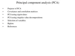
Principal Component Analysis (PCA) or Empirical Orthogonal Functions (EOFs). Arnaud Czaja (SPAT Data analysis lecture Nov. 2011). Outline. Motivation Mathematical formulation (on the board) Illustration: analysis of ~100yr of sea surface temperature fluctuations in the North Atlantic

Principal Component Analysis (PCA) or Empirical Orthogonal Functions (EOFs)
E N D
Presentation Transcript
Principal Component Analysis (PCA) or Empirical Orthogonal Functions (EOFs) Arnaud Czaja (SPAT Data analysis lecture Nov. 2011)
Outline • Motivation • Mathematical formulation (on the board) • Illustration: analysis of ~100yr of sea surface temperature fluctuations in the North Atlantic • How to compute EOFs • Some issues regarding EOF analysis
Motivation 12 EOFs • Data compression ...to “carry less luggage” Original pictures 6 EOFs 24 EOFs
Motivation QG model (231 var.) 20-EOF model • Data compression... to simplify with the hope of better understanding and forecasting Mean Z300 (CI=100m) Mean Z300 (CI=100m) Selten (1995) r.m.s Z300 (CI=10m) r.m.s Z300 (CI=10m)
Motivation • Identify “modes” empirically from data “Annular modes” in pressure data Thompson and Wallace (2000)
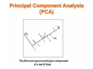
Pictures EOF2 EOF3 EOF1 Mean “picture”
North Atlantic sea surface temperature variability (Deser and Blackmon 1993) EOF2 12% EOF1 45% PC1 PC2
How to compute EOFs • Compute the covariance matrix Σ of the observation matrix X • Compute its eigenvalues (variance explained) and eigenvectors (=eof) • The principal component is then obtained by “projection”: pc(t) = X * eof • Another (more efficient) method: singular value decomposition of X (come and see me if you are interested)
Main issues with EOF analysis • Sensitivity to size of dataset (“sampling” issues) See North et al. (1982)
Main issues with EOF analysis • Sensitivity to size of dataset (“sampling” issues)
Main issues with EOF analysis • Sensitivity to size of dataset (“sampling” issues)
Main issues with EOF analysis • Orthogonality constraint is not physical. Methods have been developed to deal with this (“rotated EOFs”) • The link between EOFs and physical modes of a system is not clear
Main issues with EOF analysis • Orthogonality constraint is not physical. Methods have been developed to deal with this (“rotated EOFs”) • The link between EOFs and physical modes of a system is not clear • Good luck if you try EOFs... Do not hesitate to come and see me!