Implicit modeling and surface reconstruction
Implicit modeling and surface reconstruction. Implicit models. Algebraic surfaces Algebraic methods define surfaces with polynomial functions of three variables. Typically, these are low degree polynomials (2 to 4).

Implicit modeling and surface reconstruction
E N D
Presentation Transcript
Implicit models • Algebraic surfaces • Algebraic methods define surfaces with polynomial functions of three variables. Typically, these are low degree polynomials (2 to 4). • The most popular algebraic surfaces are surfaces with polynomials of degree 2 or so-called “quadrics” (sphere, cylinder, cone, ellipsoid, etc.). • They can be used as separate shapes or as initial primitives in Constructive Solid Geometry
Implicit models • Skeleton-based implicit surfaces • A surface is considered as a zero set of the scalar field generated by some “skeleton” field source (discrete set of points, lines, triangles, etc.). • Combining individual field functions of skeletal elements can be implemented with algebraic sum or integration technique (convolution surfaces). • Skeleton-based implicit surfaces • A skeleton-based implicit surface is defined as follows: with where is a field function of an individual skeletal element, is distance between a given point and the k-th skeletal element, and is a threshold value. Figureillustrates the simplest case of the point skeleton.
Implicit models • Convolution surfaces • Convolution surface is a generalization of skeleton-based implicit surfaces. A field function for a convolution surface is obtained by spatial convolution between a skeletal element and a Gaussian-type kernel: where X is a vector of point coordinates, S(X) is a predicate function defining geometry of the skeletal element ( for points of the element and for other points in space), h(X) is a convolution kernel.
Implicit models • Real function representation • The function representation (or F-rep) defines a whole geometric object by a single real-valued continuous function of several variables as F(X)0. F-rep combines together many different models like algebraic and skeleton based implicits • Modeling concepts include sets of objects, operations and relations. • The main restriction of well-known min/max operations is that they are C1 discontinuous. This can yield unexpected results in further operations on the object. • Any operation has to be closed on the representation, i.e., generate a continuous real function as a result. Set-theoretic operations are closed on F-rep with the use of - C k continuous R-functions: for the intersection of two objects described by f1 and f2, and for the union. These functions have C1 discontinuity only in the points where f1 = f2 = 0.
Implicit models • Real function representation • Example • Defining a “reasonable” boundary shape of the restoration area: (a) Control points of concave polygon. (b) Result of set-theoretic subtraction. • A convex polygon can be represented as the intersection of half-planes. Then, to convert this set-theoretic representation to a single real function one can use min/max or more complex R-functions. A concave polygon needs to be represented by set-theoretic operations on convex polygons or half-planes.
Implicit models • Real function representation • The monotone formula approach discussed in the next section provides the defining function without internal and external zeroes. • (a) A concave polygon with the segment S25 used for the cell partition; (b) the surface of the defining function constructed for the separation example (a); (c) a contour map of the surface (b) for the non-negative function values with “internal zeroes”; (d) a contour map of a function without “internal zeroes” generated using a monotone formula.
Implicit models • Real function representation • A counter-clockwise ordered sequence of coordinates of polygon vertices A1(x1, y1), A2(x2, y2),..., An(xn, yn) serves as the input. Also coordinates are assigned to a point An+1 (xn+1,yn+1) coincident with A1 (x1,y1). It is obvious that the equation defines a line passing through points Ai(xi,yi) and Ai+1(xi+1, yi+1); fi is a function positive in an open region and negative in an open region located respectively to the left and to the right of the line. When the region is bounded by a convex polygon, it can be given by the logical formula If is an external region of a convex polygon then
Implicit models • Real function representation • Consider a concave polygon shown in Figure a and a tree representing its monotone formula in Figure b. • In practice, the monotone formula construction results in a tree structure
Implicit models • Real function representation (example) • Generation of depth data and synthetic relief carving • Depth (height) data are extensively used in cutting simulation, digital terrain modeling, prototyping and computer vision. We apply our approach here to generate depth data from a polygonal contour. Then we apply these data to model the process of carving an arbitrary solid. • To define depth data in the functional form z = h(u,v) we construct a monotone formula for the given polygonal contour. The resulting defining function F(u,v) has positive values inside the contour, zero values on the contour and negative values outside the contour. So, we can model depth data by assigning h(u,v) = 0, if F(u,v) < 0 and h(u,v) = k F(u,v), if F(u,v) 0, where k > 0 is a scaling coefficient. Values of the function h(u,v) can be calculated at grid points and stored in a two-dimensional array.
Implicit models • Real function representation (example) • Generation of depth data and synthetic relief carving • Figure(a) shows the original image. The polygonal contour was taken from, the depth data generated from the contour (Figure(b)) and its application in carving (Figure (c)). We model relief carving with the “offsetting along the normal” operation defined as follows: G’(X) = G(X + hN), • where X = (x,y,z), G(X) is a defining function of an arbitrary three-dimensional solid, N is a gradient vector of the function G in X, h = h(T(X)) defined by ( ), and T(X) is a mapping of X onto the uv-plane. In this case, we use the parallel projection as a mapping. Figure (c) shows the result of this carving operation with the depth data in Figure (b).
Implicit models • Operations. Offsetting along normal • (a) Initial “Horse” model • (b) Offset model
Implicit models Real function representation (REFERENCES) [1] Bajaj C., Ihm I., Warren J. Higher order interpolation and least-squares approximation using implicit algebraic surfaces, ACM Transactions on Graphics, Vol. 11, No. 4, 1992, pp. 327-347. [2] Blinn J.F. A generalization of algebraic surface drawing, ACM Transactions on Graphics, Vol. 1, No. 3, 1982, pp.235-256. [3] Dischler J.-M., Ghazanfarpour D. A geometrical based method for highly complex structured textures generation, Computer Graphics Forum, Vol. 14, No. 4, 1995, pp.203-215. [4] Dobkin D., Guibas L., Hershberger J., Snoeyink J. An efficient algorithm for finding the CSG representation of a simple polygon, SIGGRAPH’88, Computer Graphics, Vol. 22, No. 4, 1988, pp.31-40. [5] Dobkin D.P., Souvaine D.L. Computational geometry in a curved world,Algorithmica, vol.5, 1990, pp.421-457. [6] Hoffmann C. On the separability problem of real functions and its significance in solid modeling, Computational Algebra, Lecture Notes in Pure and Applied Mathematics, vol.151, Marcel Dekker, 1993, pp.191-204. [7] Jones M.W., Chen M. A new approach to the construction of surfaces from contour data, EUROGRAPHICS'94, Computer Graphics Forum, Vol. 13, No. 3, 1994, pp.75-84. [8] Lim C., Turkiyyah G., Ganter M., Storti D. Implicit reconstruction of solids from cloud point sets, Third Symposium on Solid Modeling and Applications, C.Hoffmann and J.Rossignac (Eds.), 1995, pp. 393-402. [9] Muraki S. Volumetric shape description of range data using ‘blobby’ model, SIGGRAPH’91, Computer Graphics, Vol. 25, No. 4, 1991, pp. 227-235. [10] Pasko A., Adzhiev V., Sourin A., Savchenko V. Function representation in geometric modeling: concepts, implementation and applications, The Visual Computer, vol.11, No.8, 1995, pp.429-446. See also http://www.u-aizu.ac.jp/public/www/labs/sw-sm/FrepWWW/F-rep.html [11] Peterson D. Halfspace representation of extrusions, solids of revolution, and pyramids, SANDIA Report SAND84-0572, Sandia National Laboratories, Albuquerque, NM, 1984. [12] Preparata F.P., Shamos M. I. Computational Geometry: An Introduction, Springer-Verlag, New York, 1985. [13] Ricci A. A constructive geometry for computer graphics, The Computer Journal, Vol. 16, No. 2, 1973, pp. 157-160. [14] Rvachev V.L. Methods of Logic Algebra in Mathematical Physics, NaukovaDumka, Kiev, 1974.
Implicit models • Real function representation (REFERENCES) [15] Savchenko V.V., Pasko A.A. Collision detection for functionally defined deformable objects, Implicit Surfaces’95, Eurographics Workshop Proceedings, B.Wyvill and M.-P. Gascuel (Eds.), INRIA, 1995, pp. 217-221. [16] Savchenko V., Pasko A. Reconstruction from contour data and sculpting 3D objects, Journal of Computer Aided Surgery, Vol. 1, Suppl., Proceedings of Second International Symposium on Computer Aided Surgery ISCAS’95, 1995, pp.56-57. [17] V. Shapiro. Real functions for representation of rigid solids, Computer Aided Geometric Design, Vol. 11, No. 2, 1994, pp. 151-160. [18] Shapiro V., Vossler D.L. Separation for boundary to CSG conversion, ACM Transactions on Graphics, Vol. 12, No. 1, 1993, pp.35-55. [19] Singh K., Parent R. Polyhedral shapes as general implicit surface primitives, Technical Report OSU-CISRC-5/94-TR24, Ohio State University, 1994. [20] Sourin A.I., Pasko A.A. Function representation for sweeping by a moving solid, IEEE Transactions on Visualization and Computer Graphics, Vol. 2, No.1, 1996, pp.11-18. [21] Tor S.B., Middleditch A.E. Convex decomposition of simple polygons, ACM Transactions on Graphics, Vol. 3, No. 4, 1984, pp.244-265. [22] Velho L., Terzopoulos D., Gomes J. Constructing implicit shape models from boundary data, Graphical Models and Image Processing, Vol. 57, No. 3, 1995, pp.220-234. [23] Woodwark J.R., Wallis A.F. Graphical input to a Boolean solid modeller, CAD 82, A.Pipes (Ed.), Brighton, U.K., 1982, pp.681-688. [24] Wyvill G., McPheeters C., Wyvill B. Data structure for soft objects, The Visual Computer, Vol. 2, No. 4, 1986, pp.227-234.
Example: Designing a lens • Designing a lens by hand or by trial and error is a time-consuming and tedious task. A dream of the end user is to define desired photometric distribution and geometric constrains to design automatically an optical shape satisfying them • Requirements or constrains become more and more difficult to be met using traditional optimization techniques because analytical solutions do not exist for complicated shapes • In techniques based on the error functional minimization, the question may occur to solve highly non-linear problems
Example: Designing a lens (Cont.) • The issue of optimal design for optical systems for functionally represented geometric objects has not yet been addressed • We focus on an approach to modeling shapes through the use of evolutionary optimization or genetic algorithms for functionally represented geometric objects • The motivation is - to describe a case study of a “Trilobite eye” and “four-eyed” fish - to discuss problems of using the optimization procedure
RELATED WORKS J. Loos, Ph. Slusallek, H.-P. Seidel, Using wavefront tracing for the visualization and optimization of progressive lenses, EUROGRAPHICS’98, Computer Graphics Forum, vol.17, No. 3, 1998, 255-265 J. Loos, G. Greiner, H.-P. Seidel, A variational approach to progressive lens design, Computer-Aided Design, vol. 30, No. 8, 1998, 595-602 M. Halstead, B. Barsky, S. Klein, R. Mandell, Reconstructing curved surfaces from specular reflection patterns using spline surface fitting of normals. SIGGRAPH 96 Conference Proceedings, August 1996, 335-342
RELATED WORKS M. Goel, R.L. Thompson, The evolution of the trilobite eye, Computer Simulations of Self-Organization in Biological Systems, part 11, 1988, 275-290 M.I. Sobel , Light, 1987 V.V. Savchenko, A.A. Pasko, Transformation of functionally defined shapes by extended space mappings, The Visual Computer, vol. 14, Nos. 5/6, 1998, 257-270 J.H. Holland, K.J. Holyoak , R.E. Nisbett, P.R. Thagard , Induction: Processes of Inference Learning and Discovery, 1986
SHAPE MODELING SCHEME for Trilobite eye • Phacopids had eyes containing large biconvex lenses made of durable minerals. • The lens consists of two subunits separated by a concave surface
SHAPE MODELING SCHEME for Trilobite eye (Cont.) • It has a spherical upper surface of radius R1and a spherical lower surface (“bowl”) of radius R2 • Between these two surfaces, there is an intermediate refracting surface that turns the lens shape into a non-manifold object • The shape of the lens allows any light ray passing from point f1 through the lens to hit focus f2 • The region above the lens has a refractive index of n1 , and the region below the lens has a refractive index of bodily fluid of n4. The lens subunits have different refractive indexes: n2for the upper lens and n3for the lower lens • We would like to reconstruct the refracting surface using the combination of the ray tracing technique, functionally based shape modeling and GAs
VOLUME MODELING for shape reconstruction • Set-theoretic and many other operations have found quite general solutions for geometric solids represented by continuous real functions as f(x,y,z) >= 0 • There are several reasons for using this representation in optical shape design: • Shapes can be designed as combinations of analytically defined geometric objects and volumetric ones that can be obtained from measurements of natural objects • Spline-controlled global and local deformations are supported • The point membership relation based on the three-valued predicate lets us quite easily extend applications to non-manifold objects with intermediate refracting surfaces • Parametrized constructive solids (e.g., a lens with holes of variable shapes and positions) can be modeled and optimized
VOLUME MODELING for shape reconstruction (Cont.) • Naturally, approximation of the curved refractive interface by linear segments can cause C1 discontinuities in the defining function. • Using polynomial approximation we have to be cautious about high-order interpolation and errors depending on closeness of the point x to the point xi. • To provide a more smooth surface and a C1 continuous defining function, we use least square fitting to approximate a sequence of the points (xi,zi), i = 1,2, ... 12 by the Fourier series. The unknown refractive interface is described as z(x) = b0 +b1 cos(x) + b2cos(2x) + b3cos(3x) + a1 sin(x) + a2sin(2x) + a3sin(3x)
The FUNCTIONAL MODEL of the phacopid eye 1. Lens(xt,zt){ 2. shift = Fz(xt); //refractive interface 3. vf1 = sphere(xt,0,zt,R1); //upper sphere 4. vf2 = sphere(xt,0,zt,R2); //lower sphere 5. f_fi = vf1 & vf2; //intersection of spheres 6. f_fo = f_fi & (zt-shift); //upper lens unit 7. f_so = f_fi & (shift-zt); //lower lens unit 8. f_glob = f_fo | f_so; //union of two lens units //Assign a tag for point membership identification 9. if(f_fo >= 0.) id_obj = 0; 10. if(f_so >= 0.) id_obj = 1; 11. if(f_glob < 0.) id_obj = 2; 12. return f_glob;}
The FUNCTIONAL MODEL of the phacopid eye • To provide a more smooth surface and a C1 continuous defining function, we use least square fitting to approximate a sequence of the points (xi,zi), i = 1,2, ... 12 by the Fourier series • The problem of the curved refractive interface design concerns the main feature of the eye to focus a series of light rays emanating at many angles qk from a point f1 to another point f2 • The z-intercept of a light ray can be calculated by tracing the ray emanating from f1 • We calculate a “fitness” function that expresses the well-known fact that the more effectively the lens can focus lights from f1 to f2 the less residual of z-intercepts from the fixed position of focus f2 we can attain
RESULT of evolutionary optimization of the refractive interface
CASE STUDY of the “four-eyed” fish • The “four-eyed” fish, swims along the water surface with its head partly out of water, and each of its two eyes has two pupils, one kept above the surface, the other below • Each pupil focuses light upon a different retina
Surfaces. Problems 2 Fundamental Problems ∕ \ ReconstructionSegmentation of surfaces (onto a uniform grid) of surfaces into different from sparse depth measurements surface types for object that may have outliers. recognition & refinement of the surface estimates. Contours → 2-D Surfaces → 3-D
Surfaces. Problems (Cont.) • Basic methods include • Converting point measurements into a mesh of triangular facets, • Segmenting range measurements into simple surface patches, • Fitting a smooth surface to the point measurements, and • Matching a surface model to the point measurements.
Surfaces. Problems (Cont.) • One of the interpolation methods is based on the use of radial basis functions (proposed by V. Savchenko ) • Reconstruction from 3D scattered data(“Phobos” project, 1986)
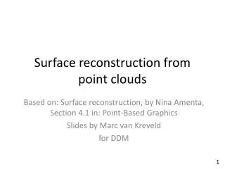
Reconstruction and Representation of 3D Objects with Radial Basis Functions Carr et al. SIGGRAPH 2001
Problem • Given a set of points • Define an implicit function , such that: • Surface is defined by the zero set of f
Constrains • f(x) = 0 is a trivial solution • Add off-surface normal points to constrain the solution further • Both side approach was proposed by Turk & O’Brien in 2001
Off-Surface Normal Points • For each point, add two more points defining the inside and outside
Off-Surface Normal Points • Create points • New constrains
Choice of Parameters • is chosen as the distance of the new point from , signed distance function • must be chosen such that the displacement to the new point doesn’t intersect other parts of the surface
Generating Normals • Input is a point cloud, no normals • Generate normals as per [Hoppe 92] • Estimation from plane fitted to neighborhood • Additionally, use consistency and/or scanner positions to resolve ambiguities • If fails, don’t define off-surface normal points
Find the Implicit Function • Given a set of distinct nodes and a set of function values , find an interpolant s, such that
The interpolant is choose from , the Beppo-Levi space of distributions on with square integrable second derivatives • Square integrable means • is the space of functions in whose second derivatives fall off quickly
Radial Basis Functions • [Duchon 77] shown that the smoothest intepolant in is • It is a particular example of Radial Basis Functions:
Radial Basis Functions • p(x) is a low degree polynomial • are real coefficients • || is the Euclidean norm in • , the basis function, is a real function • Thin plate spline function • Guassian • Biharmonic and triharmonic splines
Radial Basis Functions • For biharmonic spline RBF, • B is symmetric and invertible under very mild conditions
Non-Compact Support • Biharmonic spline RBF • Pros • Suitable to non-uniformly sample data • Handle holes • Cons • A is not sparse, more computation and not scalable
Fast Methods • Approximated with Fast Multipole Method (FMM) • Cluster RBF centers into a hierarchy • Approximate evaluation for cluster far away • Direct evaluation for clusters near by • Reduce both storage and computation
RBF Center Reduction • Use fewer centers to achieve desired accuracy • A greedy algorithm • 1. Choose a subset of centers, fit a RBF • 2. Evaluate the residual, • 3. If < desired accuracy then stop • 4. Add new centers where is large • 5. Refit RBF and goto step 2
Noisy Data • Consider both interpolation and smoothness • measures the smoothness, is the weight • The linear system changes to
Noisy Data RBF approximation of a noisy LIDAR data
Surface Evaluation • A marching tetrahedra variant, optimized for surface following • Avoid RFS evaluation at a grid of voxels • Start from several seed points • Wavefronts of facets spread out across surfaces • Stop when intersect the bounding box