Surface reconstruction from point clouds
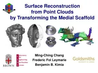
Surface reconstruction from point clouds. Based on: Surface reconstruction, by Nina Amenta , Section 4.1 in: Point-Based Graphics Slides by Marc van Kreveld for DDM. Surface reconstruction. Converting a point cloud in a more explicit representation, like a triangle mesh

Surface reconstruction from point clouds
E N D
Presentation Transcript
Surface reconstruction from point clouds Based on: Surface reconstruction, by Nina Amenta, Section 4.1 in: Point-Based Graphics Slides by Marc van Kreveld for DDM
Surface reconstruction • Converting a point cloud in a more explicit representation, like a triangle mesh • Needs a dense enough point set • especially in areas with much detail • especially in areas with high curvature • Sometimes outliers must be dealt with • Many different approaches
Surface reconstruction • Often begins with normal estimation at all points • Basic method types: • Implicit surface methods • Voronoi/Delaunay methods • Surface evolution methods
Implicit surface methods • Voxel-based method of Hoppe et al. (1992) • Estimate normal at each point p of the set P • Make all normals point outwards • Define f(x) to be the distance to the tangent plane of p, where p is the point of P closest to x • Use marching cubes to extract the zero-set of f
Implicit surface methods • Voxel-based method of Hoppe et al. (1992) • Estimate normal at each point p of the set P • Make all normals point outwards • Define f(x) to be the distance to the tangent plane of p, where p is the point of P closest to x • Use marching cubes to extract the zero-set of f within the 3D Voronoi cell of p, the surface is the tangent plane at p !
Implicit surface methods • Voxel-based method of Hoppe et al. (1992) • Estimate normal at each point p of the set P • Make all normals point outwards • Define f(x) to be the distance to the tangent plane of p, where p is the point of P closest to x • Use marching cubes to extract the zero-set of f within the 3D Voronoi cell of p, the surface is the tangent plane at p ! f is a discontinuous function !
Implicit surface methods • Exact computation of the zero-set of f involves computing the 3D Voronoi diagram of P and intersecting each cell with the local tangent plane • Hoppe et al. use marching cubes which can take care of many of the (smaller) gaps between pieces of surface
Implicit surface methods • Marching cubes algorithm (Lorensen and Cline, 1987) • method to determine the level-0 set of an implicit function • uses a grid of cubes and evaluates the function only at the corners • from the eight corners of each cube and their status inside/outside (function is negative/positive), a piece of surface is made inside the cube
Implicit surface methods • Marching squares (for level-5 set) • Four corners give 16 cases; twoare ambiguous all inside all outside
Implicit surface methods • Locally, we cannot know how to resolve an ambiguous case
Implicit surface methods • Marching cubes is the 3D equivalent idea • Eight corners of the square give 256 cases, many of which are symmetric or inverted 15 cases remain
Implicit surface methods • Two cubes that share an ambiguous facet must use compatible solutions: imagine case 3 (2 red and 6 blue vertices) and its inverted form (6 red and 2 blue vertices) share an ambiguous facet
Implicit surface methods • A solution was given by Nielson and Hammann (1991), called asymptotic decider • It includes different ways to treat certain inverted forms (so they are not inverted but new cases)
Implicit surface methods • Instead of choosing the surface to go through the middle of an edge with an inside and an outside endpoint, it is better to use interpolation (linear) f(.) = –2 let surface intersect the edge here f(.) = 5
Implicit surface methods • Back to Hoppe et al.’s voxel-based method and how marching cubes (squares) applies • Estimate normal at each point p of the set P • Make all normals point outwards • Define f(x) to be the distance to the tangent plane of p, where p is the point of P closest to x • Use marching cubes to extract the zero-set of f
Implicit surface methods • Hoppe et al.’s method resolves the gaps resulting from discontinuities in the implicit function • It can give holes in the reconstruction
Implicit surface methods • Hoppe et al.’s method, missing step: outward normal orientation: • make a Euclidean minimum spanning tree EMST on all points • find the topmost point in the EMST and make it the root of the tree • orient the root so that its normal is upwards (dot product with vertical upward direction is positive) • pre-order traverse the spanning tree and assign the normal of a node by letting it be consistent with its parent (their dot product should be positive)
root flip 1st flip 2nd flip 4th flip 5th flip 3rd
Implicit surface methods • Hoppe et al.’s method, missing step: outward normal orientation: • make a Euclidean minimum spanning tree on all points • Take all n choose 2 pairs of points and sort them by distance • Start with n points as sets with only one element • Loop over the point pairs by increasing distance: accept a pair as an edge in the EMST if the points are in different sets, then unite their sets (stop when there is only one set) • we can take only the pairs of points whose Voronoi cells are neighbors (typically fewer than quadratically many)
Implicit surface methods • Hoppe et al.’s method: outward normal orientation: • Problem: the method may make mistakes when sampling is low near areas with high curvature
Implicit surface methods • Hoppe et al.’s method: outward normal orientation: • Problem: the method may make mistakes when sampling is low near areas with high curvature • Solution: • First make a graph G where every point is connected to its k nearest neighbors (k is a small constant to be chosen) • Give every edge a weight depending on to what extent the normals are parallel (including inverted): 1 – [the absolute value of the dot product of the normalized normalsat these points] • Compute the minimum spanning tree of G using these weights [ normalized = scaled to have unit length ]
Implicit surface methods • All of this works in 3D too • Note that in 3D the desired spanning tree will not have such a simple path structure as you would expect in 2D
Implicit surface methods • More advanced: Let f be composed of the sum of many “local” implicit functions fi, one for each pi • These local implicit functions are blended into f • The weight wi of fiat a point x depends on the distance between x and pi; it decreases monotonically with the distance • The weights must make an unbiased interpolator/ estimator of the local implicit functions
Implicit surface methods • The functions fi could be chosen as in Hoppe et al.: the signed distance to the normal plane at pi • The weights wi can also be chosen to be a linear fall-off function, or a Gaussian fall-off function • If for any point x, f(x) isinfluenced by only few fi(with weight wi > 0), thenthe surface can be recon-structed efficiently • In Gaussian case, use cut-off wi distance
Voronoi and Delaunay methods • The Voronoi diagram and Delaunay triangulation of a set of points sampled on a surface have a lot of structure that can be used for reconstruction
Reconstructing with Delaunay • Possibilities: • Let the object be the union of Delaunay triangles (2D) or tetrahedra (3D) that are deemed to be inside the shape • Decide of edges (2D) or triangles (3D) that they are part of the boundary of the shape α-shape
Reconstructing with Voronoi • Possibilities: • Use the Voronoi diagram to estimate normals as the diameters of the Voronoi cells • Extract the medial axis from the Voronoi diagram of the points; it resembles the medial axis of the reconstruction
The α-shape • The α-shape is a general shape descriptor for a set of points [ Edelsbrunner, Kirkpatrick, Seidel 1983]
The α-shape • The α-shape is the straight-line graph with the α-extreme points as the vertices and the α-neighbors as the edges α-neighbors radius α-disk α-extreme point
The α-shape • Every α-shape edge is also a Delaunay triangulation edge (it has an empty circle through its endpoints) α-neighbors radius α-disk α-extreme point
The α-shape • The choice of αis important • bigger α: avoids holes and separate components in shape, but also less detail • smaller α: more detail but risk of holes and separate components • How to determine the right α? • Can we make α adaptive: smaller where point density is higher and larger where point density is lower?
The α-shape • We can compute the 2D α-shape from the Delaunay triangulation by testing every edge: determine the radius of the smallest and largest empty circle through its endpoints Circles containing p and q have their centers on the bisector of p and q p Empty circles containing p and q have their centers between the centers of the circumcircles of the two triangles incident to edge pq q
The α-shape p largest q p This center realizes the smallest circle This center realizes the smallest circle q largest

