Download
1 / 35
380 likes | 624 Vues
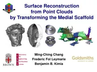
Ming-Ching Chang Frederic Fol Leymarie Benjamin B. Kimia. Surface Reconstruction from Point Clouds by Transforming the Medial Scaffold. Problem: surface reconstruction with minimal assumptions. Context: reconstruct a surface mesh from unorganized

E N D
Ming-Ching Chang Frederic Fol Leymarie Benjamin B. Kimia Surface Reconstructionfrom Point Clouds by Transforming the Medial Scaffold
Problem: surface reconstruction with minimal assumptions • Context: reconstruct a surface mesh from unorganized • points, with a “minimal” set of assumptions: the samples are nearby a “possible” surface(thick volumetric traces not considered here). • Benefit: reconstruction across many types of surfaces.
Goal: surface reconstruction with minimal assumptions To find a general approach, applicable to various topologies, without assuming strong input constraints, e.g.: • No surface normal information. • Unknown topology (with boundary, for a solid, with holes, non-orientable). • No a priori surface smoothness assumptions. • Practical sampling condition: non-uniformity, with varying degrees of noise. • Practical large input size (> millions of points).
Goal: surface reconstruction with minimal assumptions • Surface normal : not accurate, or problem locally solved • Unknown topology : practical (e.g., holes, in CAD) • No smoothness : practical (sharp features) • Non-uniformity, noise : practical acquisition • Large input size : scalable
How: Literature Overview • Implicit distance functions • Locally approximate the distance function by blending primitives. • Globally approximate the distance function by volumetric propagation. • Propagation based (region growing) methods • Voronoi / Delaunay geometric constructs • Incremental surface-oriented. • Volume-oriented. • Many methods have additional assumptions in addition to unorganized points: • Surface normal: imply knowing the surface locally. • Surface enclose a volume (distance field): a strong global information.
How we solve it: Find an Inverse of Sampling: • Relate the sampled surface with the underlying (unknown) surface and try to invert (recover) the sampling process…
How: Overview of Our Approach (2D) Not many clues from the assumed loose input constraints. • Work on the shape itself to recover the sampling process. • Key ideas: • Relate the sampled shape with the underlying (unknown) surface by a sequence of shape deformations (growing from samples). • Represent (2D) shapes by their medial “shock graphs”. [Kimia et al.] • Handle shocktransitions across different shock topologies to recover gaps.
How: Sampling / Meshing as Deformations Schematic view of sampling: infinitesimal holes grows, remaining are the samples. We consider the removing of a patch from the surface as a Gap Transform. 2D: 3D:
How: Medial Scaffolds for 3D Shapes A graph structure for the 3D Medial Axis • Classify shock points into 5 general types, and organized into a hyper-graph form [Giblin, Kimia PAMI’04]: • Shock Sheet: A12 • Shock Curves: A13 (Axial), A3 (Rib) • Shock Vertices: A14, A1A3 Akn: contact (max. ball) at n distinct points, each with k+1 degree of contact. A special case of input of points the Medial Scaffold consists of only: A12Sheets, A13Curves, A14Vertices. A14 Vertex A12 Sheet A13 Curve
How: Medial Scaffolds for 3D Shapes A graph structure for the 3D Medial Axis • Augmented Medial Scaffold (MS+): hyper-graph [Leymarie PAMI’07]: • Reduced Medial Scaffold (MS): 1D graph structure • Shock sheets are seen as redundant (loops in the graph). Easter island statue point data courtesy of Yoshizawa et al.
How: Organise/Order Deformations (2D) A B NB: A & B share object symmetries. Symmetries due to the sampling need to be identified. Deformation in shape space
How: Organise/Order Deformations (3D) • Recover a mesh (connectivity) structure by usingMedial Axistransitionsmodelled via the Medial Scaffold (MS). • Meshing as shape deformations in the ‘shape space’. • The Medial Scaffold of a point cloud includes both the symmetries due to sampling and the original object symmetries. • Rank order Medial Scaffold edits (gaptransforms) to “segregate” and to simulate the recovery of sampling. Sampling recovery Object symmetry Meshed Surface + Organized MA Shock Segregation [Leymarie, PhD’02]
Algorithmic Method Enough theory… Here is how we order symmetries (and thus gap transforms) in practice.
Three A12 shock sheets G1 G1 G3 A13-2 singular shock point G1 G0 G2 G0 G2 G0 G2 A13-2 Type I Type II Type III Algorithmic Method • Consider Gap Transforms on allA13 shock curves in a ranked-order fashion: • best-first (greedy) with error recovery. • Cost reflects: • Likelihood that a shock curve (triangle) represents a surface patch. • Consistency in the local context (neighboring triangles). • Allowable (local surface patch) topology. A13 shock curve 3 Types of A13 shock curves (dual Delaunay triangles): Represented in the MS by “singular shock points” (A13-2) (unlikely to be correct candidate)
Algorithmic Method How we order gap transforms: • Favor small “compact” triangles. • Favor recovery in “nice” (simple) areas, e.g., away from ridges, corners, necks. • Favor simple local continuity (similar orientation). • Favor simple local topologies (2D manifold). • BUT: allow for error recovery!
R R unbounded Ranking Isolated Shock Curves (Triangles) Triangle geometry: (Heron’s formula) (Compactness, Gueziec’s formula, 0<C<1) Cost: favors smallcompact triangles with large shock radius R. The side of smaller shock radius is more salient. R: minimum shock radius dmax: maximum expected triangle, estimated from dmed Surface meshed from confident regions toward the sharp ridge region.
A13-2 Estimate the Sampling Scale The maximum expected triangle size (dmax) can be estimated from shock radius distribution analysis. Distribution of the A13-2 radii of all shock curves corresponding to: All triangles of shock curves of type I and type II in the (full) Medial Scaffold of the point cloud. All triangles in the original Stanford bunny mesh. The median of the A13-2 distribution (dmed) approximates its peak.
Cost Reflecting Local Context & Topology Cost to reflect smooth continuity of edge-adjacent triangles: Typology of triangles sharing an edge: Typology of mesh vertex topology Point data courtesy of Ohtake et al.
Strategy in the Greedy Meshing Process Queue of ordered triangles Problem: Local ambiguous decisions errors. Solutions: • Multi-pass greedy iterations First construct confident surface triangles without ambiguities. • Postpone ambiguous decisions • Delay related candidate Gap Transforms close in rank, until additional supportive triangles (built in vicinity) are available. • Delay potential topology violations. • Error recovery • For each Gap Transform, re-evaluate cost of both related neighboring (already built) & candidate triangles. • If cost of any existing triangle exceeds top candidate, undo itsGap Transform.
Summary of Our Approach • We relate an object and its sampling by navigating the “shape space” (of deformations). • We organize this navigation by gap transforms on the Medial Scaffold. • We select a path by ordering these transforms and allowing for error recovery.
Show Time! • Some results • Other issues: • Validation, • Using a priori information, • Dealing with large inputs, • Sampling quality, • Running time. • Conclusions
Results: Surface with Various Types Non-orientable Water-tight surface With sharp ridges (discontinuous curvature) With boundary Multiple components With multiple holes Multiply punctured Closely knotted Gold: water-tight surface: Blue: mesh boundary. Dataset are courtesy of Cyberware, Stanford data repository, Stony Brook archive, H. Hoppe.
Result: Videos on Meshing Algebraic Surfaces Mobius strip Costa minimum surface (courtesy of H. Hoppe)
Result: Video on Meshing the Rocker Arm Flat smooth regions are meshed prior to the ridges/corners. The rocker arm data courtesy of Cyberware.
Validation • Superimpose our meshing result on the original mesh. Color: Original mesh in gray. Difference of reconstructed triangles in green.
Other Issues • Validation, • Using a priori information, • Dealing with large inputs, • Sampling quality, • Running time.
Re-mesh / Repair a Partial Mesh • In the case that existing triangles (in addition to the points) are know a priori: • Assign high priority to existing triangles. • Let candidates compete in the greedy algorithm. • Similar if surface normal is available. RESULTS Meshing result of an implementation of ball pivoting algorithm (BPA) containing holes / topological errors. 4,102 points sampling a mechanical part (courtesy of H. Hoppe) Re-mesh results of our algorithm (a solid)
Handle Large Datasets (Millions of Points) • No strong constraints (topology, boundary, volume, etc.) on input. • Divide input into buckets (or any full partition of space). • Mesh surfaces in each bucket. • Stitch surfaces by applying the same algorithm again. Meshing Stanford Asian Dragon (3.6M points). Related to [Dey et al.’01]: Super Cocone.
Result: Bucketing + Stitching Video 120,965 points, divided into 20,000 points per bucket. Sapho dataset courtesy of Stony Brook archive.
Dealing with sampling quality Input of non-uniform and low-density sampling: Response to additive noise: 50% 100% 150%
Surface Meshing Running Time • Roughly linear to the number of samples. • Performance similar to other recent Delaunay filtering methods.
Conclusions • Surface reconstruction from point clouds. • Handle a great variety of surfaces of practical interest. • With little restrictions on input. • Mesh surface by applying min. costGap Transforms in best-first manner, considering: • Geometrical suitability of candidate Delaunay triangles. • Shock type, shock curve radius. • Continuity from neighbors. • Mesh topology. • Multiple-pass greedy algorithm with error recovery. • Potential to handle arbitrarily large datasets.
Future Work & Discussions • Additional Shock Transforms to handle allshock transitions. • Better greedy error recovery. • Medial Axis regularization: application to shape manipulation, segmentation, recognition. • Surface meshing: theoretical guarantees. Medial Scaffold (MS+) Corresponding surface patches Regularized MS+ Acknowledgments: Support from NSF. Coin3D (OpenInventor) for visualization/GUI. Stanford, Cyberware, MPII, Stony Brook archive for 3D data.