Atmospheric Soundings, Surface Properties, Clouds
Atmospheric Soundings, Surface Properties, Clouds. The Bologna Lectures Paul Menzel NOAA/NESDIS/ORA. Relevant Material in Applications of Meteorological Satellites CHAPTER 6 - DETECTING CLOUDS 6.1 RTE in Cloudy Conditions 6-1

Atmospheric Soundings, Surface Properties, Clouds
E N D
Presentation Transcript
Atmospheric Soundings, Surface Properties, Clouds The Bologna Lectures Paul Menzel NOAA/NESDIS/ORA
Relevant Material in Applications of Meteorological Satellites CHAPTER 6 - DETECTING CLOUDS 6.1 RTE in Cloudy Conditions 6-1 6.2 Inferring Clear Sky Radiances in Cloudy Conditions 6-2 6.3 Finding Clouds 6-3 CHAPTER 7 - SURFACE TEMPERATURE 7.2. Water Vapor Correction for SST Determinations 7-3 7.3 Accounting for Surface Emissivity in the Determination of SST 7-6 7.4 Estimating Fire Size and Temperature 7-6 CHAPTER 8 - TECHNIQUES FOR DETERMINING ATMOSPHERIC PARAMETERS 8.1 Total Water Vapor Estimation 8-1 8.3 Cloud Height and Effective Emissivity Determination 8-8 8.6 Satellite Measurement of Atmospheric Stability 8-13
Earth emitted spectra overlaid on Planck function envelopes O3 CO2 H20 CO2
Profile Retrieval from Sounder Radiances ps I = sfc B(T(ps)) (ps) - B(T(p)) [ d(p) / dp ] dp . o I1, I2, I3, .... , In are measured with the sounder P(sfc) and T(sfc) come from ground based conventional observations (p) are calculated with physics models First guess solution is inferred from (1) in situ radiosonde reports, (2) model prediction, or (3) blending of (1) and (2) Profile retrieval from perturbing guess to match measured sounder radiances
Sounder Retrieval Products Direct brightness temperatures Derived in Clear Sky 20 retrieved temperatures (at mandatory levels) 20 geo-potential heights (at mandatory levels) 11 dewpoint temperatures (at 300 hPa and below) 3 thermal gradient winds (at 700, 500, 400 hPa) 1 total precipitable water vapor 1 surface skin temperature 2 stability index (lifted index, CAPE) Derived in Cloudy conditions 3 cloud parameters (amount, cloud top pressure, and cloud top temperature) Mandatory Levels (in hPa) sfc 780 300 70 1000 700 250 50 950 670 200 30 920 500 150 20 850 400 100 10
Remote Sensing Regions Windows to the atmosphere (regions of minimal atmospheric absorption) exist near 4 m and 10 m; these are used for sensing the temperature of the earth surface and clouds. CO2 absorption bands at 4.3 m and 15 m are used for temperature profile retrieval; because these gases are uniformly mixed in the atmosphere in known portions they lend themselves to this application. The water vapor absorption band near 6.3 m is sensitive to the water vapor concentration in the atmosphere; as H20 is not uniformly mixed in the atmosphere, measurements in this spectral region are used to infer moisture distribution in the atmosphere. The ozone absorption band at 9.7 m reveals locations of O3 concentration in the upper atmosphere.
Comparison of GOES-8 PW with microwave retrievals GOES Sounder total precipitable water (PW) values compare well with co-located microwave radiometer measurements at the CART site (Lamont, OK). “Flat” first-guess trace is adjusted by sounder radiances to capture the trend and range of total moisture.
Comparison of GOES-8 PW with microwave retrievals A scatter plot comparing MWR integrated water vapor values and GOES-8 first guess/physical retrieval values at the CART site . RMS and bias values for all matches are quantified in the lower right hand corner.
Interactive Viewing of GOES Sounder DPI Time Series UW/Madison/CIMSS NOAA/NESDIS/ORA/ARAD/ASPT (de-stabilizing with time) (example from Dec. 2, 1999) (graph lines: thick when sounding available, thin when cloud obscured) A new interactive web site (http://cimss.ssec.wisc.edu/goes/realtime/gdpiviewer.html) allows users to view time series of GOES derived product imagery (Lifted Index (LI), Precipitable Water (PW), and Convective Available Potential Entergy (CAPE)) by clicking on a desired location within the latest Derived Product Image (DPI).
Detecting Clouds (IR) IR Window Brightness Temperature Threshold and Difference Tests IR tests sensitive to sfc emissivity and atm PW, dust, and aerosols BT11 < 270 BT11 + aPW * (BT11 - BT12) < SST BT11 + bPW * (BT11 - BT8.6) < SST aPW and bPW determined from lookup table as a function of PW BT3.9 - BT11 > 12 indicates daytime low cloud cover BT11 - BT12 < 2 (rel for scene temp) indicates high cloud BT11 - BT6.7 large neg diff for clr sky over Antarctic Plateau winter CO2 Channel Test for High Clouds BT13.9 < threshold (problems at high scan angle or high terrain)
Detecting Clouds (vis) Reflectance Threshold Test r.87 > 5.5% over ocean indicates cloud r.66 > 18% over vegetated land indicates cloud Near IR Thin Cirrus Test r1.38 > threshold indicates presence of thin cirrus cloud ambiguity of high thin versus low thick cloud (resolved with BT13.9) problems in high terrain Reflectance Ratio Test r.87/r.66 between 0.9 and 1.1 for cloudy regions must be ecosystem specific Snow Test NDSI = [r.55-r1.6]/ [r.55+r1.6] > 0.4 and r.87 > 0.1 then snow
1.6 µm image 0.86 µm image 11 µm image 3.9 µm image cloud mask Snow test (impacts choice of tests/thresholds) 11 - 12 BT test (primarily for high cloud) VIS test (over non-snow covered areas) 13.9 µm high cloud test (sensitive in cold regions) 3.9 - 11 BT test for low clouds aa MODIS cloud mask example (confident clear is green, probably clear is blue, uncertain is red, cloud is white)
AVIRIS Movie #2 AVIRIS Image - Porto Nacional, Brazil 20-Aug-1995 224 Spectral Bands: 0.4 - 2.5 mm Pixel: 20mx 20mScene: 10km x 10km
MODIS identifies cloud classes
Clouds separate into classes when multispectral radiance information is viewed
Multispectral data reveals improved information about ice / water clouds
Cloud Composition Contrails Image Over Kansas - 21 April 1996 Ice Cloud Infrared Temperature Difference - 8.6 m (Band 29) - 11.0 m (Band 31) Contrails Water Cloud Infrared Temperature Difference - 11.0 m (Band 31) - 12.0 m (Band 32)
Tri-spectral IR thermodynamic phase algorithm ice cloud April 1996 Success • 8.6-11 vs 11-12 • when slope > 1 then ice • when slope < 1 then water water cloud Jan 1993 TOGA/ COARE Strabala, Menzel, and Ackerman, 1994, JAM, 2, 212-229. Baum et al, 2000, JGR, 105, 11781-11792.
RTE in Cloudy Conditions Iλ = η Icd + (1 - η) Ic where cd = cloud, c = clear, η = cloud fraction λ λ o Ic = Bλ(Ts) λ(ps) + Bλ(T(p)) dλ . λ ps pc Icd = (1-ελ) Bλ(Ts) λ(ps) + (1-ελ) Bλ(T(p)) dλ λ ps o + ελ Bλ(T(pc)) λ(pc) + Bλ(T(p)) dλ pc ελ is emittance of cloud. First two terms are from below cloud, third term is cloud contribution, and fourth term is from above cloud. After rearranging pc dBλ Iλ - Iλc = ηελ(p) dp . ps dp Techniques for dealing with clouds fall into three categories: (a) searching for cloudless fields of view, (b) specifying cloud top pressure and sounding down to cloud level as in the cloudless case, and (c) employing adjacent fields of view to determine clear sky signal from partly cloudy observations.
Cloud Clearing For a single layer of clouds, radiances in one spectral band vary linearly with those of another as cloud amount varies from one field of view (fov) to another Clear radiances can be inferred by extrapolating to cloud free conditions. clear RCO2 x partly cloudy xx x x x x cloudy x x N=1 N=0 RIRW
Paired field of view proceeds as follows. For a given wavelength λ, radiances from two spatially independent, but geographically close, fields of view are written Iλ,1 = η1 Iλ,1cd + (1 - η1) Iλ,1c , Iλ,2 = η2 Iλ,2 cd + (1 - η2) Iλ,2c , If clouds are at uniform altitude, and clear air radiance is in each FOV Iλcd = Iλ,1cd = Iλ,2 cd Iλc = Iλ,1c = Iλ,2c cd c c η1 (Iλ - Iλ ) η1 Iλ,1 - Iλ = = η* = , cd c c η2 (Iλ - Iλ) η2 Iλ,2 - Iλ where η* is the ratio of the cloud amounts for the two geographically independent fields of view of the sounding radiometer. Therefore, the clear air radiance from an area possessing broken clouds at a uniform altitude is given by c Iλ = [ Iλ,1 - η* Iλ,2] /[1 - η*] where η* still needs to be determined. Given an independent measurement of surface temperature, Ts, and measurements Iw,1 and Iw,2 in a spectral window channel, then η* can be determined by η* = [Iw,1 - Bw(Ts)] / [Iw,2 - Bw(Ts)] and Iλc for different spectral channels can be solved.
Cloud Properties RTE for cloudy conditions indicates dependence of cloud forcing (observed minus clear sky radiance) on cloud amount () and cloud top pressure (pc) pc (I - Iclr) = dB . ps Higher colder cloud or greater cloud amount produces greater cloud forcing; dense low cloud can be confused for high thin cloud. Two unknowns require two equations. pc can be inferred from radiance measurements in two spectral bands where cloud emissivity is the same. is derived from the infrared window, once pc is known. This is the essence of the CO2 slicing technique.
Moisture Moisture attenuation in atmospheric windows varies linearly with optical depth. - ku = e = 1 - k u For same atmosphere, deviation of brightness temperature from surface temperature is a linear function of absorbing power. Thus moisture corrected SST can inferred by using split window measurements and extrapolating to zero k Ts = Tbw1 + [ kw1 / (kw2- kw1) ] [Tbw1 - Tbw2] . Moisture content of atmosphere inferred from slope of linear relation.
Early SST algorithms * IRW histogram of occurrence f of observed brightness temperatures T f(T) = fs exp [ -(T - Tsfc)2/22 ] instrument noise / scene variability produce Gaussian distribution; warm side of histogram reveals Ts = T(d2f/dT2=0) - * Three point method combinations of (Ti, fi), (Tj, fj), and (Tk, fk) on the warm side of the histogram enable 3 equations / 3 unknowns, hence a histogram of Ts solutions. * Least squares method ln (f(T)) = ln (fs) - Ts2/22 + TsT/2 - T2/22 has the form ln (f(T)) = Ao + A1T + A2T2 , so Ts = - A1/(2A2) .
Histograms of infrared window brightness temperature in cloud free and cloud contaminated conditions
Water Vapor Correction for SST Determinations * Water vapor correction (T) Ts = Tb + T ranges from 0.1 C in cold/dry to 10 K in warm/moist atmospheres for 11 um IRW observations. * Water vapor correction is highly dependent on wavelength. * Water vapor correction depends on viewing angle. * In IRW for small water vapor concentrations, w = e-Kwu ~ 1 - Kwu so that Ts = Tbw1 + [ Kw1 / (Kw2- Kw1) ] [Tbw1 - Tbw2] . linear extrapolation to moisture free atmosphere * Regression of clear sky IRW obs and collocated buoys create current operational algorithm Ts=A0+A1* Tbw1 +A2*( Tbw1-Tbw2)+A3*(Tbw1-Tbw2)2 a quadratic term helps account for occasional large water vapor concentrations.
Cloud Detection • Several multispectral methods have evolved to detect clouds in the area of interest. • Input data are vis, T3.9, T11, and T12 , T11@30min, • and SST guess. • General tests include: • T11 > 270 K ocean rarely frozen • T11 > T12 + 4 K clouds affect moisture correction • vis < 4% clouds reflect more than ocean sfc • T11 - T3.9 > 1.5 K subpixel clouds • T11 < 0.3 K SST over 1 hr small • -2 K < SST- guess < 5 K SST over days bounded
Advantages of Geostationary SST Estimates * 10 times more observations of a given location * multispectral cloud detection supplemented by temporal persistence checks * clear sky viewing enhanced by persistence (e.g. can wait for clouds to move through) * daily composite provides good spatial coverage * can discern diurnal excursions in SST * can track SST motions as estimates of ocean currents
GOES daily composite SST reveals small scale features in oceans
Accounting for surface emissivity When the sea surface emissivity is less than one, there are two effects that must be considered: (a) the atmospheric radiation reflects from the surface, and (b) the surface emission is reduced from that of a blackbody. The radiative transfer can be written ps I = B(Ts) (ps) + B(T(p))d(p) o ps + (1-) (ps) B(T(p))d‘(p) o where ‘(p) represents the transmittance down from the atmosphere to the surface. This can be rewritten I = B(ps)(ps) + B(TA)[1 - (ps) - (ps)2 + (ps)2] . Note that as the atmospheric transmittance approaches unity, the atmospheric contribution expressed by the second term becomes zero.
HIS and GOES radiance observations plotted in accordance with the radiative transfer equation including corrections for atmospheric moisture, non-unit emissivity of the sea surface, and reflection of the atmospheric radiance from the sea surface. Radiances are referenced to 880 cm-1. The intercept of the linear relationship for each data set represents a retrieved surface skin blackbody radiance from which the SST can be retrieved.
Comparison of ocean brightness temperatures measured by a ship borne interferometer (AERI), by an interferometer (HIS) on an aircraft at 20 km altitude, and the geostationary sounder (GOES-8). Corrections for atmospheric absorption of moisture, non-unit emissivity of the sea surface, and reflection of the atmospheric radiance from the sea surface have not been made.
GOES 3 by 3 FOVs (30 km) 11 micron MODIS 5 by 5 FOVs (5 km)
5km resolution MODIS 500hPa T 30km resolution GOES
GOES vs. MODIS 2000/06/30 1600 UTC Total Precipitable Water (mm)
GOES vs. MODIS 2000/06/30 1600 UTC Total Precipitable Water (mm) MODIS 5 km resolution TPW TPW GOES 30 km resolution