Introduction to Color
Introduction to Color. Spectral color: single wavelength (e.g., from laser); “ROY G. BIV” spectrum Non-spectral color: combination of spectral colors; can be shown as continuous spectral distribution or as discrete sum of n primaries (e.g., R, G, B); most colors are non-spectral mixtures

Introduction to Color
E N D
Presentation Transcript
Spectral color: single wavelength (e.g., from laser); “ROY G. BIV” spectrum Non-spectral color: combination of spectral colors; can be shown as continuous spectral distribution or as discrete sum of n primaries (e.g., R, G, B); most colors are non-spectral mixtures Metamers are spectral energy distributions that are perceived as the same “color” each color sensation can be produced by an arbitrarily large number of metamers Energy Distribution and Metamers White light spectrum where the height of the curve is the spectral energy distribution Cannot predict average observer’s color sensation from a distribution
Metamers (1/4) Different light distributions that produce the same response • Imagine a creature with just one kind of receptor, say “red,” whose response curve looks like this: • How would it respond to each of these two light sources? • Both signals will generate the same amount of “red” perception. Hence they are metamers • one type of receptor can never give us more than one color sensation, red in this case • although, different signals may result in different perceived brightness
Metamers (2/4) • Consider a creature with two receptors (R1, R2) • Note that in principle an infinite number of frequency distributions can simulate the effect of I2, e.g., I1 • in practice, for In near base of response curves, amount of light required becomes impractically large I1 I1 I2
Metamers (3/4) • For three types of receptors, there are potentially infinitely many color distributions (metamers) that will generate exactly the same sensations • you can test this out with the metamer applet • we’ll do this in lab • Conversely, no two spectral (monochromatic) lights can generate identical receptor responses and therefore all look unique • Thomas Young in 1801 postulated that we need 3 types of receptors to distinguish the gamut of colors represented by triples H, S and V Metamer Applet http://www.cs.brown.edu/exploratories/freeSoftware/repository/edu/brown/cs/exploratories/applets/spectrum/metamers_guide.html
Metamers (4/4) • For two light sources to be metamers, the amounts of red, green, and blue response generated by the two sources must be identical • This amounts to three constraints on the lights • But the light sources are infinitely variable – one can adjust the amount of light at any possible wavelength… • So there are infinitely many metamers • Observations: • if two people have different response curves, the metamers for one person will be different from those for the other • metamers are purely perceptual: scientific instruments can detect the difference between two metameric lights • even a prism can help show how two metameric lights are different…
Spectral color: single wavelength (e.g., from laser); “ROY G. BIV” spectrum Non-spectral color: combination of spectral colors; can be shown as continuous spectral distribution or as discrete sum of n primaries (e.g., R, G, B); most colors are non-spectral mixtures Metamers are spectral energy distributions that are perceived as the same “color” each color sensation can be produced by an arbitrarily large number of metamers Energy Distribution and Metamers White light spectrum where the height of the curve is the spectral energy distribution Cannot predict average observer’s color sensation from a distribution
Can characterize visual effect of any spectral distribution by triple (dominant wavelength, excitation purity, luminance): Dominant wavelength corresponds to hue we see; spike of energy e2 Excitation purity is the ratio of monochromatic light of the dominant wavelength and white light to produce the color e1 = e2, excitation purity is 0% (unsaturated) e1 = 0, excitation purity is 100% (fully saturated) Luminance relates to total energy, which is proportional to integral of the product of distribution and eye’s response curve (“luminous efficiency function”) – depends on both e1 and e2 Note: dominant wavelength of a real distribution may not be the one with the largest amplitude! some colors (e.g., purple) have no dominant wavelength e2 Dominant Wavelength Energy Density e1 Idealized uniform distribution except for e2 wavelength, nm 400 700 Colorimetry Terms
Receptors in retina (for color matching) rods and three types of cones (tristimulus theory) primary colors (only three used for screen images: approximately red, green, blue (RGB)) Note: the 3 types of receptors each respond to a wide range of frequencies, not just three spectral primaries Opponent channels (for perception) other cells in retina and neural connections in visual cortex blue-yellow, red-green, black-white 4 psychological color primaries*: red, green, blue, and yellow Opponent cells (also for perception) spatial (context) effects, e.g., simultaneous contrast, lateral inhibition * These colors are called “psychological primaries” because each contains no perceived element of the others regardless of intensity. (www.garys-gallery.com/colorprimaries.html) Three Layers of Human Color Perception – Overview
Receptors contain photopigments that produce electro-chemical response; our dynamic range of light, from a few photons to looking at the sun, is 1011 => division of labor among receptors Rods (scotopic): only see grays, work in low-light/night conditions, mostly in periphery Cones (photopic): respond to different wavelength to produce color sensations, work in bright light, densely packed near fovea, center of retina, fewer in periphery Young-Helmholtz tristimulus theory1: 3 types of cones, each sensitive to all visible wavelengths of light, each maximally responsive in different ranges, often associated with red, green, and blue (although red and green peaks of these cones actually more yellow) The three types of receptors can produce a 3-space of hue, saturation and value (lightness/brightness) To avoid misinterpretations S (short), I (intermediate), L (long) often used instead Receptors in Retina 1Thomas Young proposed the idea of three receptors in 1801. Hermann von Helmholtz looked at the theory from a quantitative basis in 1866. Hence, although they did not work together, the theory is called the Young-Helmholtz theory since they arrived at the same conclusions.
Tristimulus theory does not explain color perception, e.g., not many colors look like mixtures of RGB (violet looks like red and blue, but what about yellow?) Triple Cell Response Applet: http://www.cs.brown.edu/exploratories/freeSoftware/repository/edu/brown/cs/exploratories/applets/spectrum/triple_cell_response_guide.html Tristimulus Theory Spectral-response functions of fλ each of the three types of cones on the human retina
Additional neural processing the three receptor elements have both excitatory and inhibitory connections with neurons higher up that correspond to opponent processes; one pole of each activated by excitation, the other by inhibition All colors can be described in terms of 4 “psychological color primaries” R, G, B, and Y However, a color is never reddish-greenish or bluish-yellowish: leads to idea of two “antagonistic” opponent color channels, red-green and yellow-blue a third, black and white channel, relays lightness information S I L - + + + + + + - + BK-W Y-B R-G Hering’s Chromatic Opponent Channels Light of 450 nm Each channel is a weighted sum of receptor outputs – linear mapping Hue: Blue + Red = Violet
Some cells in the opponent channels are also spatially opponent, a type of lateral inhibition (called double-opponent cells) Responsible for effects of simultaneous contrast and after images green stimulus in cell surround causes some red excitement in cell center, making gray square in field of green appear reddish Plus… color perception strongly influenced by context, training, etc., not to mention abnormalities such as various types of color blindness Spatially Opponent Cells
Nature provides for contrast enhancement at boundaries between regions: edge detection. This is caused by lateral inhibition. Mach Bands and Lateral Inhibition A Stimulus intensity B Position on stimulus
Lateral Inhibition and Contrast Two receptor cells, A and B, are stimulated by neighboring regions of a stimulus. A receives an intense amount of light. A’s excitation serves to stimulate the next neuron on the visual chain, cell D, which transmits the message further toward the brain. But this transmission is impeded by cell B, whose own intense excitation exerts an inhibitory effect on cell D. As as result, cell D fires at a reduced rate. (Excitatory effects are shown by green arrows, inhibitory ones by red arrows.) Intensity of cell cj=I(cj) is a function of cj’s excitation e(cj) inhibited by its neighbors with attenuation coefficients ak that decrease with distance. Thus, At the boundary more excited cells inhibit their less excited neighbors even more and vice versa. Thus, at the boundary the dark areas are even darker than the interior dark ones, and the light areas are lighter than the interior light ones.
Color Matching • Tristimulus theory leads to notion of matching all visible colors with combinations of “red,” “green,” and “blue” mono-spectral “primaries;” it almost works • Note: these are NOT response functions! • Negative value of => cannot match, must “subtract,” i.e., add that amount to unknown • Note that mixing positive amounts of arbitrary R, G, B primaries provides large color gamut, e.g., CRT, but no device based on a finite number of primaries can show all colors! Wavelength λ (nm) Color-matching functions, showing the amounts of the three primaries needed by the average observer to match a color of constant luminance, for all values of dominant wavelength in the visible spectrum.
CIE Space for Color Matching • Commission Internationale de l´Éclairage (CIE) • Defined X, Y, and Z primaries to replace red, green and blue primaries => RGBinXYZi via a matrix The mathematical color matching functions xλyλ, and zλ for the 1931 CIE X, Y, and Zprimaries. They are defined tabularly at 1 nm intervals for color samples that subtend 2° field of view on retina
Note the irregular shape of the visible gamut in CIE space; it is due to the eye's response as measured by the response curves The range of colors which can be displayed on the monitor is clearly smaller than all colors visible in XYZ space. CIE Space Showing an RGB Gamut The color gamut for a typical color monitor with the XYZ color space
Left: the plane embedded in CIE space. Top right: a view perpendicular to the plane. Bottom right: the projection onto the (X, Y) plane (that is, the Z = 0 plane), which is called the chromaticity diagram Chromaticity – Everything that deals (H, S) with color, not luminance/brightness For an interactive chromaticity diagram, check out the following applet: http://www.cs.rit.edu/~ncs/color/a_chroma.html CIE Space Projection to Chromaticity Diagram Several views of the X + Y+ Z = 1 plane of the CIE space
Amounts of X, Y, and Z primaries needed to match a color with a spectral energy distribution P(λ), are: in practice use S’s Then for a given color C, C = XX + YY + ZZ Get chromaticity values that depend only on dominant wavelength (hue) and saturation (purity), independent of the amount of luminous energy, for a given color, by normalizing for total amount of luminous energy = (X + Y + Z) thus x + y + z = 1; (x,y,z) lies on the X + Y + Z = 1 plane CIE Chromaticity Diagram (1/5)
(x, y) determinesz but cannot recover X, Y, Z from only x and y. Need one more piece of information, typically Y, which carries luminance information Then CIE Chromaticity Diagram (2/5)
CIE chromaticity diagram is the projection onto the (X, Y) – plane of the (X + Y + Z ) = 1 plane It plots x and y for all visible chromaticity values: all perceivable colors with same chromaticity but different luminances map into same point 100% spectrally pure, monochromatic colors are on curved part since luminance factored out, colors that are luminance-related are not shown, e.g., brown = orange-red chromaticity at low luminance infinite number of planes which project onto (X + Y + Z = 1) plane and all of whose colors differ; thus it is NOT a full color palette! illuminant C: near (but not at) x = y = z = 1/3; close to daylight CIE Chromaticity Diagram (3/5) spectral locus not the spectral locus
Uses of CIE Chromaticity Diagram: Name colors Define color mixing Define and compare color gamuts CIE Chromaticity Diagram (4/5)
CIE Chromaticity Diagram (5/5) CIE 1976 UCS chromaticity diagram from Electronic Color: The Art of Color Applied to Graphic Computing by Richard B. Norman, 1990 Inset: CIE 1931 chromaticity diagram
Measure dominant wavelength and excitation purity of any color by matching with mixture of the three CIE primaries: colorimeters measure tristimulus X, Y, and Z values from which chromaticity coordinates are computed spectroradiometers measures the wavelengths of both spectral energy distribution and tristimulus values Suppose matched color is at point A in figure below: when two colors added, new color lies on straight line connecting two colors => A = tC + (1– t)B where B is a spectral color ratio AC/BC is excitation purity of A Using the CIE Chromaticity Diagram (1/2) Colors portrayed on the chromaticity diagram
Complementary colors can be mixed to produce white light (a decidedly non-spectral color!); white can thus be produced by an approximately constant spectral distribution as well as by only two complementary colors, e.g., greenish-blue, D, and reddish-orange,E (on previous slide). Some nonspectral colors (colors not on the spectral locus, like G) cannot be defined by dominant wavelength; defined by complementary dominant wavelength Using the CIE Chromaticity Diagram (2/2)
As we saw, any two colors, I and J, can be added to produce any color along their connecting line by varying relative amounts of two colors in mix Third color K can be used with various mixes of I and J to produce a gamut of all colors in triangle IJK, again by varying relative amounts Shape of diagram shows why visible red, green and blue cannot be additively mixed to match all colors; no triangle whose vertices are within the visible area can completely cover visible area (e.g., purple and magenta) matching of all visible colors requires negative amounts of primaries for some due to the way response curves overlap and sum Color Gamuts (1/2) Mixing colors
Color Gamuts (2/2) • Smallness of print gamut with respect to color monitor gamut => faithful reproduction by printing must use reduced gamut of colors on monitor
No gamut described by a linear combination of n physical (real) primaries (yielding aconvex hull) can simulate the eye’s responses to all visible colors Review of CIE shape of CIE space determined by the Matching Experiment: subject is shown a color and asked to create a metameric match out of three colored monochromatic primaries, R, G and B most colors can be matched, but some can’t because of the way the response curves are overlapped would need “negative amounts” of one of the primaries in order to match all visible color samples; not physically possibly, but can be simulated by adding that color to the sample to be matched. to simplify, the CIE mathematical primaries, X, Y, and Z, are used to get all positive color matching functions Let’s see in another way why 3 (indeed n) physical primaries aren’t sufficient to match an arbitrary color by looking at the response function Why the Chromaticity Diagram is Not Triangular
Here we try to match a monospectral cyanish color (440nm) with our three red, green, and blue lights. We show the three response function, labeled S, I, and L and try two different R, G, B intensity triples Match Failure Example try to match spectral light at 440 nm Three R, G, B primaries Height of bar shows amplitude of primary
Taken from Falk’s Seeing the Light, Harper and Row, 1986 Chromatic Opponent Channels on Chromaticity Diagram
Purpose: specify colors in some gamut Since gamut is a subset of all visible chromaticities, model does not contain all visible colors 3D color coordinate system subset containing all colors within a gamut Means to convert to other model(s) Example color model: RGB 3D Cartesian coordinate system unit cube subset Use CIE XYZ space to convert to and from all other models Color Models for Raster Graphics (1/2)
Hardware-oriented models: not intuitive – do not relate to concepts of hue, saturation, brightness RGB, used with color CRT monitors YIQ, the broadcast TV color system CMY (cyan, magenta, yellow) for color printing CMYK (cyan, magenta, yellow, black) for color printing User-oriented models HSV (hue, saturation, value) – also called HSB (hue, saturation, brightness) HLS (hue, lightness, saturation) The Munsell system CIE Lab Color Models for Raster Graphics (2/2)
RGB primaries are additive: The RGB cube (Grays are on the dotted main diagonal) Main diagonal => gray levels black is (0, 0, 0) white is (1, 1, 1) RGB color gamut defined by CRT phosphor chromaticities differs form one CRT to another The RGB Color Model (1/3)
Conversion from one RGB gamut to another convert one to XYZ, then convert from XYZ to another check out http://www.color3d.com/examples.htm for some good examples of this Form of each transformation: Where Xr, Xg, and Xb are the weights applied to the monitor’s RGB colors to find X, and so on M is the 3 x 3 matrix of color-matching coefficients Let M1 and M2 be matrices to convert from each of the two monitor’s gamuts to CIE M2-1 M1 converts form RGB of monitor 1 to RGB of monitor 2 The RGB Color Model (2/3)
But what if C1 is in the gamut of monitor 1 but is not in the gamut of monitor 2, i.e., C2 = M2-1 M1C1 is outside the unit cube and hence is not displayable? Solution 1: clamp RGB at 0 and 1 simple, but distorts color relations Solution 2: compress gamut on monitor 1 by scaling all colors from monitor 1 toward center of gamut 1 ensure that all displayed colors on monitor 1 map onto monitor 2 The RGB Color Model (3/3)
Used in electrostatic and in ink-jet plotters that deposit pigment on paper Cyan, magenta, and yellow are complements of red, green , and blue Subtractive primaries: colors are specified by what is removed or subtracted from white light, rather than by what is added to blackness Cartesian coordinate system Subset is unit cube white is at origin, black at (1, 1, 1): Green Yellow (minus blue) (minus red) Cyan Black Red Blue Magenta (minus green) The CMY(K) Color Model (1/2) • subtractive primaries (cyan, magenta, yellow) and their mixtures
Color printing presses, some color printers use CMYK (K=black) K used instead of equal amounts of CMY called undercolor removal richer black less ink deposited on paper – dries more quickly First approximation – nonlinearities must be accommodated: K = min(C, M, Y) C’ = C – K M’ = M – K (one of C’, Y’, M’ will be 0) The CMY(K) Color Model (2/2)
Recoding for RGB for transmission efficiency and downward compatibility with B/W broadcast TV; used for NTSC (National Television Standards Committee (cynically, “never the same color”)) Y is luminance – same as CIE Y primary I and Q encode chromaticity Only Y = 0.3R + 0.59G + 0.11B shown on B/W monitors: weights indicate relative brightness of each primary assumes white point is illuminant C: xw = 0.31, yw = 0.316, and Yw = 100.0 Preparing color material which may be seen on B/W broadcast TV, adjacent colors should have different Y values NTSC encoding of YIQ: 4 MHz Y (eye most sensitive to r luminance) 1.5 MHz I (small images need only 1 color dimension) 0.6 MHz Q The YIQ Color Model
Hue, saturation, value (brightness) Hexcone subset of cylindrical (polar) coordinate system Single hexcone HSV color model. (The V = 1 plane contains the RGB model’s R = 1, G = 1, B = 1, in the regions shown) Has intuitive appeal of the artist’s tint, shade, and tone model pure red = H = 0, S = 1, V = 1; pure pigments are (I, 1, 1) tints: adding white pigment n decreasing S at constant V shades: adding black pigment n decreasing V at constant S tones: decreasing S and V The HSV Color Model (1/2)
Colors on V = 1 plane are not equally bright Complementary colors 180° opposite Saturation measured relative to color gamut represented by model which is subset of chromaticity diagram: therefore, 100% S 100% excitation purity Top of HSV hexcone is projection seen by looking along principal diagonal of RGB color RGB subcubes are plane of constant V Code for RGB n HSV on page 592, 593 Note: linear path RGB linear path in HSV! The HSV Color Model (2/2) RGB color cube viewed along the principal diagonal
Hue, lightness, saturation Double-hexcone subset Maximally saturated hues are at S = 1, L = 0.5 Less attractive for sliders or dials Neither V nor L correspond to Y in YIQ! Conceptually easier for some people to view white as a point The HLS color Model
They are perceptually non-uniform move through color space from color C1 to a new color C1΄through a distance ΔC C1΄ = C1 + ΔC move through the same distance ΔC, starting from a different color C2 C2΄ = C2 + ΔC the change in color in both cases is mathematically equal, but is not perceived as equal Moving a slider almost always causes a perceptual change in the other two parameters, which is not reflected by changes in those sliders; thus, changing hue frequently will affect saturation and value, even in Photoshop! Ideally want a perceptually uniform space: two colors that are equally distant are perceived as equally distant, and changing one parameter does not perceptually alter the other two Historically, the first perceptually-uniform color space was the Munsell system Problems with Standard Color Systems
Created from perceptual data, not as a transformation of or approximation to CIE Uniform perceptually-based 3D space accounts for the fact that a bright yellow is much lighter than a bright blue, and that many more levels of saturation of blue can be distinguished than of yellow Magnitude of change in one parameter always maps to the same effect on perception Hues arranged on a circle a 20 degree rotation through this circle always causes the same perceptual change, no matter where on the circle you start from does not cause changes in saturation or value Saturation as distance from center of circle moving away from the center a certain distance always causes the same perceptual change does not cause changes in hue or value Value as height in space moving vertically always causes the same perceptual change does not cause changes in hue or saturation Basis for Graphics Group research during 1999-2001 into new color pickers (was led by ams and funded by Adobe) The Munsell System
CIE Lab was introduced in 1976 popular for use in measuring reflective and transmissive objects Three components: L* is luminosity a* is red/green axis b* is yellow/blue axis Mathematically described space and a perceptually uniform color space Given white = (Xn, Yn, Zn) These transformations cause regions of colors perceived as identical to be of the same size CIE Lab
RGB + Cartesian coordinate system + linear + hardware-based (easy to transform to video) + tristimulus-based - hard to use to pick and name colors - doesn’t cover gamut of perceivable colors - non-uniform: equal geometric distance => unequal perceptual distance CIE + covers gamut of perceived colors + based on human perception (matching experiments) + linear + contains all other spaces - non-uniform (but variations such as CIE Lab are closer to Munsell, which is uniform) - xy-plot of chromaticity horseshoe diagram doesn’t show luminance Color Model Pros and Cons (1/2)
Example: Photoshop Lab color model is based on CIE Lab space + based on psychological colors (y-b, r-g, w-b) - terrible interface in Photoshop - no visualization of the color space - very difficult to determine what values mean if you are unfamiliar with the space - picks colors which are out of the print gamut - primarily used as an internal space to convert between RGB and CMYK HSV + easy to convert to RGB + easy to specify colors - nonlinear - doesn’t cover gamut of perceivable colors - nonuniform Color Model Pros and Cons (2/2)
English-language names ambiguous and subjective Numeric coordinates in color space with slide dials: Interactive Specification of Color (1/2) Left: Lab color picker from Adobe Photoshop for Windows Below: RGB color picker from Adobe Photoshop for Mac OS
Interact with visual representation of the color space Important for user to see actual display with new color Beware of surround effect! Interactive Specification of Color (2/2) HSB color picker from Adobe Photoshop HSV color picker from Mac OS X’s Finder
Interpolation needed for: Gouraud shading antialiasing blending images together in a fade-in, fade-out sequence Results depend on the color model used: RGB, CMY, YIQ, CIE are related by affine transformations, hence straight line (i.e., interpolation paths) are maintained during mapping not so for HSV, HLS; for example, interpolation between red and green in RGB: interpolating in HSV: midpoint values in RGB differ by 0.5 from same interpolation in HSV: (60º, 1, 0.5)(60º, 1, 1) Interpolating in Color Space (1/2) • red = (1, 0, 0), green = (0, 1, 0) • midpoint = (0.5, 0.5, 0) • red = (0º, 1, 1); green = (120º, 1, 1) • midpoint = (60º, 1, 1) • RGB_to_HSV = (60º, 1, 0.5)