Controllability of feedback systems
620 likes | 954 Vues
Controllability of feedback systems. Sigurd Skogestad Department of Chemical Engineering Norwegian University of Science and Tecnology (NTNU) Trondheim, Norway Workshop: Modelling of astrocyte function June 8, 2006, University of Oslo. NTNU, Trondheim. Motivation.

Controllability of feedback systems
E N D
Presentation Transcript
Controllability of feedback systems Sigurd Skogestad Department of Chemical Engineering Norwegian University of Science and Tecnology (NTNU) Trondheim, Norway Workshop: Modelling of astrocyte functionJune 8, 2006, University of Oslo
NTNU, Trondheim
Motivation • I have co-authored a book: ”Multivariable feedback control – analysis and design” (Wiley, 1996, 2005) • What parts could be useful for system biology? • Control as a field is closely related to systems theory • Here: Focus on the use of negative feedback • Some other areas where control may contribute (Not covered): • Identification of dynamic models from data (not in my book anyway) • Model reduction • Nonlinear control (also not in my book) • Discrete event and hybrid systems (also not in my book)
Outline • Overview of control theory and concepts • Feedback • Positive and negative feedforward • Simple example: Feedforward vs. feedback • Problem feedback: (Effective) Time delay • Cascade control • Control hierarchies • Time scale separation • Controlled variables • Self-optimizing control • Summary and concluding remarks
Overview of Control theory • Classical feedback control (1930-1960) (Bode): • Single-loop (SISO) feedback control • Transfer functions, Frequency analysis (Bode-plot) • Fundamental feedback limitations (waterbed). Focus on robustness • Optimal control (1960-1980) (Kalman): • Optimal design of Multivariable (MIMO) controllers • Model-based ”feedforward” thinking; no robustness guarantees (LQG) • State-space formulation (A,B,C,D); Advanced mathematical tools (LQG) • Robust control (1980-1995) (Zames, J.C. Doyle) • Combine classical and optimal control • Optimal design of controllers with guaranteed robustness (H∞) • Nonlinear control (1950 - ) • ”Feedforward thinking”, mostly mechanical systems • Adaptive control (1970-1985) (Åstrøm) • Discrete event and hybrid systems • Automata theory • Computer science
Disturbance (d) Plant (uncontrolled system) Input (u) Output (y) Important system theoretic / control concepts • Cause-effect relationship • Classification of variables: • ”Causes” (external independent variables): Disturbances (d) and inputs (u) • ”Effects” (dependent variables): Internal states (x) and outputs (y) • Parameters (p): Internal model variables – give model uncertainty • Linear system: Parameter changes can generate instability but not disturbances • Typical state-space model used in control:
Linearized model descriptions (useful for analysis and controller design) • State space realization • Transfer function realization (input-output model) • Frequency analysis
Disturbance (d) Plant (uncontrolled system) Input (u) Output (y) Control • Active adjustment of inputs (available degrees of freedom, u) to achieve the operational objectives of the system • Most cases: Acceptable operation = ”Output (y) close to desired setpoint (ys)” ys time
Control theory Design
Control theory concepts • Steady-state = Equilibrium point = DC • Poles/modes/eigenvalues: Characteristic of dynamic response of system associated with system states • Model (= our realization of the real system): • (state) Controllability • (state) Observability • Zeros: Characteristic of dynamic response of system inverse • Stability • System maintains equilibrium point (Lyapunov stability) • Linear system (local behaviour): • Stable = eigenvalue/pole in left half plane (LHP) • Unstable = eigenvalue/pole(s) in right half plane (RHP)
Robustness • Insensitivity of system behavior to uncertainty (parameter variations) • Most real biological systems are robust • Robustness generally requires negative feedback • Measures and tools for robustness analysis • Uncertainty representation • Stability margins • Positivity, small gain theorem • Structured singular value (Doyle)
(Input-Output) Controllability • Input-output: Is the system inherently controllable? • First requirement: Stabilization • ‘‘Natural” (open-loop = without control) unstable system: • Can not be stabilized with feedforward control • Can only be stabilized by feedback • Must require that any unstable modes are detectable and stabilizable • Detectable: Unstable modes observable in the outputs • Stabilizable: Unstable modes controllable by the inputs • Next requirement: performance
Controllability limitations (performance) Serious limitations: • (Effective) Time delay in direct path from input to output • Want input close to output 2. Unstable inverse (RHP-zeros) • Limits input-output controllability because system inverse is unstable Other limitations: • Large disturbances • Small process gain (inputs weakly affect outputs) 5. Unstable system (even if unstable modes are detectable and stabilizable) 6. Nonlinearity
Fundamental limitations • Waterbed effect (”no free lunch”) for feedback control: • Does NOT apply to first-order system
Positive and negative feedback in biological systems (from Wipikedia) • Positive feedback amplifies possibilities of divergences (evolution, change of goals); it is the condition to change, evolution, growth; it gives the system the ability to access new points of equilibrium. • For example, in an organism, most positive feedbacks provide for fast autoexcitation of elements of endocrine and nervous systems (in particular, in stress responses conditions) and play a key role in regulation of morphogenesis, growth, and development of organs, all processes which are in essence a rapid escape from the initial state. Homeostasis is especially visible in the nervous and endocrine systems when considered at organism level. • Negative feedback helps to maintain stability in a system in spite of external changes. It is related to homeostasis. • Negative feedback combined with time delay can give instability: A well known example in ecology is the oscillation of the population of snowshoe hares due to predation from lynxes. • Le Chateliers principle for stable equilibrium (OK for main effect): • Systems responds by counteracting effect of disturbance
Typical chemical plant: Tennessee Eastman process Recycle and natural phenomena give positive feedback
xAs xA FA XC Control uses negative feedback
Disturbance (d) Plant (uncontrolled system) Output (y) Input (u) CONTROL • Acceptable operation = ”Output (y) close to desired setpoint (ys)” • Control: Use input (u) to counteract effect of disturbance (d) on y • Two main principles: • Feedforward control (measure d, predict and correct ahead) • (Negative) Feedback control (measure y and correct afterwards)
Disturbance (d) Plant (uncontrolled system) Output (y) Input (u) No control: Output (y) drifts away from setpoint (ys)
Setpoint (ys) Disturbance (d) Predict FF-Controller≈ Plant model-1 Plant (uncontrolled system) Offset Input (u) Output (y) • Feedforward control: • Measure d, predict and correct (ahead) • Main problem: Offset due to model error
Disturbance (d) Setpoint (ys) Input (u) Plant (uncontrolled system) FB Controller ≈ High gain e Output (y) • Feedback control: • Measure y, compare and correct (afterwards) • Main problem: Potential instability • (if we increase gain to improve performance)
k=10 time 25 Example 1 d Gd G u y Plant (uncontrolled system)
d Gd G u y
Model-based control =Feedforward (FF) control d Gd G u y ”Perfect” feedforward control: u = - G-1 Gd d Our case: G=Gd → Use u = -d
d Gd G u y Feedforward control: Nominal (perfect model)
d Gd G u y Feedforward: sensitive to gain error
d Gd G u y Feedforward: sensitive to time constant error
d Gd G u y Feedforward: Moderate sensitive to delay (in G or Gd)
Feedback (FB) control d Gd ys e=ys-y Feedback controller G u y Negative feedback: u=f(e) ”Counteract error in y by change in u’’
e=ys-y u Feedback controller Feedback (FB) control • Simplest: On/off-controller • u varies between umin (off) and umax (on) • Problem: Continous cycling
e=ys-y u Feedback controller Feedback (FB) control • Most common in industrial systems: PI-controller
d Gd G u y Back to the example
d Gd ys e C G u y Output y Input u Feedback generates inverse! Resulting output Feedback PI-control: Nominal case
d Gd ys e C G u y offset Integral (I) action removes offset
d Gd ys e C G u y Feedback PI control: insensitive to gain error
d Gd ys e C G u y Feedback: insenstive to time constant error
d Gd ys e C G u y Feedback control: sensitive to time delay
Summary example • Feedforward control is NOT ROBUST (it is sensitive to plant changes, e.g. in gain and time constant) • Feedforward control: gradual performance degradation • Feedback control is ROBUST (it is insensitive to plant changes, e.g. in gain and time constant) • Feedback control: “sudden” performance degradation (instability) Instability occurs if we over-react (loop gain is too large compared to effective time delay). • Feedback control: Changes system dynamics (eigenvalues) • Example was for single input - single output (SISO) case • Differences may be more striking in multivariable (MIMO) case
Stabilization requires feedback Output y Input u
Conclusion: Why feedback?(and not feedforward control) • Simple: High gain feedback! • Counteract unmeasured disturbances • Reduce effect of changes / uncertainty (robustness) • Change system dynamics (including stabilization) • Linearize the behavior • No explicit model required • MAIN PROBLEM • Can not have fast/tight control of plant with (effective) time delay • Potential instability (may occur “suddenly”) with time delay
Problem feedback: Effective delay θ • Effective delay PI-control = ”original delay” + ”inverse response” + ”half of second time constant” + ”all smaller time constants” • Example: Series-cascade of five first-order systems y u u y(t) t
Improve control? • Some improvement possible with more complex controller • For example, add derivative action (PID-controller) • May reduce θeff from 3.5 s to 2.5 s • Problem: Sensitive to measurement noise • Does not remove the fundamental limitation (recall waterbed) • Add extra measurement and introduce local control • May remove the fundamental waterbed limitation • Waterbed limitation does not apply to first-order system • Cascade
Engineering systems • Most (all?) large-scale engineering systems are controlled using hierarchies of quite simple single-loop controllers • Commercial aircraft • Large-scale chemical plant (refinery) • 1000’s of loops • Simple components: on-off + P-control + PI-control + nonlinear fixes + some feedforward Same in biological systems
Hierarchical structure Brain Organs Local control in cells