Download
1 / 24
240 likes | 260 Vues
12th Nordic Process Control Workshop. Controllability of Processes with Large Gains. Sigurd Skogestad Antonio C. B. de Araújo NTNU, Trondheim, Norway August, 2004. Introduction. McAvoy and Braatz (2003) (*) based on a study case with valve stiction:

E N D
12th Nordic Process Control Workshop Controllability of Processes with Large Gains Sigurd Skogestad Antonio C. B. de Araújo NTNU, Trondheim, Norway August, 2004
Introduction • McAvoy and Braatz (2003)(*) based on a study case with valve stiction: For control purposes the magnitude of steady-state process gain (maximum singular value) should not exceed about 50. • If correct, it has important implications for design of many processes. • However, seems intuitively it must be wrong: Condsider control of liquid level: Has infinite steady-state gain due to integrator, but is easily controllable • The objective of our work is to study this in more detail (*) T. A. McAvoy and R. D. Braatz, 2003, ”Controllability of processes with large singular values”, Ind. Eng. Chem. Res., 42, 6155-6165.
Claims by McAvoy and Braatz: • Systems with very high gain are sensitive. Impossible in practice to get the fine manipulation of the control valves that is required for control because the valves would be limited to move in a very small region • Upper limit for σ1(G) should be imposed. Suggest that a reasonable limit is 50 because essentially all control systems are eventually implemented with analogue devices which typically have an accuracy on the order of 0.5%. • Valve stiction: May get rid of oscillations by detuning the controller.
Study Case (McAvoy and Braatz, 2003) • Plant is given by: σ1(G) = 101.2 and σn(G) = 1.196 • ... and the controller is given by: This controller is first tuned such that KCi=0.154 and TRi=7.7s.
Study Case (McAvoy and Braatz, 2003) • The block diagram of the system was built using Simulink as follows:
uq u Study Case (McAvoy and Braatz, 2003) • Valve stiction induces a ”disturbance” at the input. • Here: Reproduce using Simulink Quantizer which discretizes the input: • Smooth signal into a stair-step output: uq = q * round(u/q), where q is the Quantization interval parameter • q=0.01: Reproduces results by McAvoy and Braatz (2003).
- With perfect valve - With valve inaccuracy y1 y2 Study Case (McAvoy and Braatz, 2003) • First we reproduce the same results as in the paper for the case where a step change of 0.23 is introduced in the setpoint of y1 and KC1 = KC2 = 0.154.
- Original tuning - Controller for y1 detuned y1 y2 Study Case (McAvoy and Braatz, 2003) • Eliminate oscillations by detuning? • Simulation with KC1 reduced by a factor 3 to0.0513: It looks very nice with no oscilation on y2. That is the orignal final time McAvoy and Braatz (2003) choose for this simulation.
- Original tuning - Controller for y1 detuned y1 y2 Study Case (McAvoy and Braatz, 2003) • Let’s make the time interval longer...... The oscilations in y2 start after about 95s. Actually, with integral action oscillations will always appear - it may just takes longer time if the controller gain is reduced
0.03 0.028 0.026 0.024 0.022 1 0.02 u 0.018 0.016 0.014 0.012 0.01 0 20 40 60 80 100 120 140 160 180 200 Study Case (McAvoy and Braatz, 2003) • This is what input 1 is doing: y1 u1 • Desired steady-state output: yss = 0.23 • Required average steady-state input: uss = yss/11 = 0.02091. • So u1must cycle between 0.02 and 0.03 (9.1% of the time)
Study Case (Skogestad and Araujo, 2004) • Consider simpler SISO example where T=0.05 or smaller. T = ”effective delay” • K(s): PI-controller that cancels dominant time constant at 1. • The Quantizer step is 1, representing an on/off valve (the ”worst-case valve”).
Study Case (Skogestad and Araujo, 2004) • Setpoint response with T=0.05 • Cycling because of integral action in controller • Average input: uss = yss/k = 1/4.1 = 0.24 (24% at 1; 76% at 0) • Magnitude of oscillations in y: a = 0.063
Study Case (Skogestad and Araujo, 2004) • Again: Magnitude and frequency of oscillations independent of controller tuning • But depend on plant dynamics; simulating for various T (effective delay): • The magnitude is clearly related to T. Why? • We need a light!!!
Relay r(t) Process u(t) y(t) Controller Relay Feedback Method • Oscillations in the outputs can be generated by relay feedback (on/off-controller). • Cycles at natural frequency Pu = 1/w180. • Furthermore, from relay formula (Åstrøm, 1988), the corresponding ultimate controller gain is where d is the relay amplitude (input) and a is the amplitude (output) of the oscillations. In our case, d = 0.5 (half of the Quantizer step)
Study Case (Skogestad and Araujo, 2004) • Relay formula • Can also find Ku from frequency domain analysis:
Controllability with inaccurate valve Inaccurate valve with quantization d: Assume that we require a < amax(max output variation). Gives controllability requirement: Gives upper limit on plant gain at frequency where L = - Note: amax=1 and d = 0.016 (1.6% valve error) gives |G(jwL180)|<50
Conclusions OK Only true for feedforward without pulsing. No problem with feedback (must accept some cycling) Only at bandwidth frequency – no limit at steady-state No. Always oscillations if controller has integral action • Systems with very high gain are sensitive. Impossible in practice to get the fine manipulation of the control valves that is required for control because the valves would be limited to move in a very small region • Upper limit for σ1(G) should be imposed. Suggest that a reasonable limit is 50 because essentially all control systems are eventually implemented with analogue devices which typically have an accuracy on the order of 0.5%. • My get rid of oscillations by detuning the controller.
Paper: Large process gain • Introduction, Previous work. Briefly mention MB-paper (1 page) • Input disturbances is main potential problem (1 page): • A. Load disturbance. |G(jwb)| < bound (previous work; easy to derive) • B. Valve inaccuracy, |G(jwL180)|< bound (have derived) • Nothing at steady-.state . Counterexample: Liquid level • A. Input load disturbance (2 pages) • Derive bound • Haig gain -> Require high bandwidth. (wb=closed-loop bandwidth) because |G(jw)| drops with w. • If not possible with high bandwidth: Must redesign • Example: pH-neutralization (ssgain = 1e6). High bw not possible. Must redesign: Add more tanks (ssgain same, but drops at high freq) • B. Valve inaccuracy (“stiction”) (6 pages) • Use new example and results from this paper • Start with example. Use example with a high gain • Theory • Always get oscillations if integral action in controller • Gain at wL180 (NOT same as wB; wB is where |L|=1; well-designed control system: very close) • Note wL180 approx wG180 because phase of controller (PI or PID) is close to zero at wG180) • Magnitude of oscillations: a = (4/pi) * |G(jwL180)| * d • NOTATION? A -> ya, E ?, d-> dq , uq ??? • This is the maximum (worst-case), likely to happen because for some operations valve is likely to be in mid-range. • Challenge: Prove that this is the MAX we get (with “fully developed” sinusoids – midrange input) • Important difference from A: Bandwidth wb (Controller gain) has no effect • So how can you avoid oscillations from inaccurate valve / stiction? • From formula: Only thing you can do is change valve (smaller dq) • or take away integral action, but must then accept offset (PROBABLY of magnitude a) • Or redesign process (put an extra tank) • Stress that controller tuning normally does not matter • Gain: no effect • Integral time: No effect if reasonably tuned • P-controller: May get rid of oscillations • Discussion (1 page) • MB-paper. Too short simulation time • “Not fully developed sinusoids” • MIMO • Conclusion
Conclusions • System with inaccurate valve (quantifier). • Controller tuning has no effect on output variations due to quantizer. Thus, detuning does NOT help, because the integral action will in any case force the system into cycling. • Magnitude of the disturbance or setpoint may have some effect, especially on Pu, due to its influence on the steady-state: • If steady-state input is reasonably in the "middle" between to quantification values and we get "fully" developed sinusoids • If steady-state is close to one of the quantification values (e.g. u = 0.21 with uq1=0.2 and uq2=0.3, then it is only f = 0.1 of the time at 0.3) then sinusoid is probably not fully developed. May try step response analysis
Singular Value Decomposition (SVD) • Antonio: ”In order to make life beautiful God created man, man has created lots of problems, and man had the brilliant idea of creating SVD to solve some of them”. • Any matrix can be decomposed into the SVD: G=UΣVH, U and V: unitary matrices Σ: diagonal matrix of of singular values σi • SVD gives useful information about input and output directions. G=UΣVH GV=UΣ Gvi= σiui, for column i. • Furthemore for any input direction v: • v1 and u1 and σ1: strong direction • vn and un and σn:: weake direction. • Condition number:
σ1(G) and σn(G) • Skogestad and Postlethwaite (1996): Need σn(G) ≥ 1 to avoid input saturation (assuming unitary scaling). • Skogestad and Postlethwaite (1996): ”A large condition number may be caused by a small valueof σn, which is generally undesirable. On the other hand, a large value of σ1 is not necessarily a problem.” • McAvoy and Braatz (2003): Also a large value of σ1 should be avoided. Their claim is based on an example (”study case”) with valve stiction
Study Case (McAvoy and Braatz - revisited) • Okay! • But what about McAvoy and Braatz- example? • Loop 1 gives us: • Observed oscillations in the output y1: a = (0.266-0.236)/2 = 0.005 with period P = 13. • Theory (relay formula): a=0.009 with period P = 1/w180 = 4 • Does not quite agree...
Study Case (McAvoy and Braat, 2003 - revisited) • Thee sinusoids are not fully developed • Give us another light, please!
Process Study Case (McAvoy and Braat, 2003 - revisited) • Try ”step response” analysis which should be better for not fully developed sinusoids. • For short response times: Approximate G as integrating process: G = 11/10s. • Response: y1(t) = (11/10)*d*t. • How long (T) does pulse last? • We need to find the fraction of time, f, T is at the maximum value (0.03). • The steady-state input is uss = yss/11 = 0.23/11 = 0.02091. • So pulse lasts 9.1% of the period of 13s. • Thus, T = 0.091*13 = 1.18s, so y(T) = (11/10)*0.005*1.18 = 0.0065 (OK!)