Download
1 / 9
90 likes | 143 Vues
Learn how to analyze Nyquist and Bode diagrams, Gain Margin, Phase Margin, and more in control system design using MATLAB.

E N D
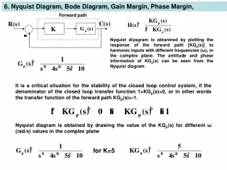
6. Nyquist Diagram, Bode Diagram, GainMargin, PhaseMargin, Forward path Nyquist diyagram is obtanined by plotting the response of the forward path [KGp(s)] to harmonic inputs with different frequencies (ω), in the complex plane. The amlitude and phase information of KGp(s) can be seen from the Nyquist diagram It is a critical situation for the stability of the closed loop control system, if the denominator of the closed loop transfer function 1+KGp(s)=0, or in other words the transfer function of the forward path KGp(s)=-1. Nyquist diagram is obtained by drawing the value of the KGp(s) for different ω (rad/s) values in the complex plane for K=5
The value of output of KGp(s) to a harmonic input having ω= 2 rad/s and amplitude of 1 can be calculated as shown below Im clc;clear w=2; s=i*w; K=5; KGp=K/(s^3+4*s^2+5*s+10) mag=abs(KGp) phas=angle(KGp)*180/pi KGp = -0.7500 - 0.2500i mag = 0.7906 phas = -161.5651 Re -0.75 -0.25 Input amplitude is 1 Output amplitude is 0.7906 0.7906
KGp(s) plane Im Nyquist diagram is drawn by connecting the tip of the vectors representing the KGp(s) for different ω frequencies. -1 Re -0.78 -0.5334 -0.75 -0.5098 -0.0201i ω=2.2 -0.25i ω=2.0 Increasing ω ω=1.8 rad/s -0.8427i ω=1.7 rad/s ω=2.2 rad/s KGp(s)=-0.5334 - 0.0201i ω=2.0 rad/s KGp(s)=-0.7500 - 0.2500i ω=1.8 rad/s KGp(s)=-0.7873 - 0.8427i ω=1.7 rad/s KGp(s)=-0.5098 - 1.1722i Nyquist curve -1.1722i
K=5; num=[K]; den=[1 4 5 10]; nyquist(num,den) Denominator of the closed loop system From Routh-Hurwitz When KGp(s)=-1, the closed loop control system is marginally stable.
Nyquist diagram Bode diagram Vector length [KGp(s)]= a Amplitude 1, decibel value 0 How many degrees there are when the vectıor length is 1? What is the value of vector length in decibel when the vector is in horizontal position.? Vector horizontal, phase -180º Vector length [KGp(s)]= 1 The relation can be used to find the critical value of the proportinal controller When the vector length of [KGp(s)] is 1, its value in logarithmic scale is zero. K KGp(s)=-a Kc KGp(s)=-1 Φ is the phase of KGp(s). When the phase angle is -180º , KGp(s) is on the real axis and its amplitude is shown as -a. When Nyquist curve intersects the real axis at -1, control system is marginaly stable. Gain Margin (gm) Gain margin in logarithmic scale
Bode diagram is the representation of the magnitude and phase of the forward path of a closed loop system KGp(s) in decibel scale for different harmonic input frequencies. Magnitude is given in decibel and phase is given in degree. The frequencies for gain and phase margin are represented by ω2 and ω1, respectively and they are calculated using Matlab as described below. clc;clear K=5; num=K*[1]; den=[1 4 5 10]; bode(num,den) [gm,pm,w2,w1]=margin(num,den) or KGp(s) clc;clear K=5; num=K*[1]; den=[1 4 5 10]; sys=tf(num,den); bode(sys) [gm,pm,w2,w1]=margin(sys) tf is a Matlab command to form the transfer function. Matlab gives the gain margin in linear scale as gm. Critical gain value Kcr can be calculated by multiplying the actual gain value K by gm. Kcr=K*gm=5*2=10 The gain margin is obtained in decibel scale from Bode diagram (GM). The relationship between GM and gm is GM=20log10(gm) gm=10GM/20 gm = 2.0024 pm = 33.2155 w2 = 2.2367 w1 = 1.8830 GM Gain margin in linear scale The closed loop system is stable if the gain curve is intersected below 0, otherwise control system is unstable. Phase margin (degree) Frequency for gain margin Damping ratio PM Frequency for phase margin ω1 ω2
Bode diagrams of first order systems Bode diagrams of second order systems Corner frequency=a (rad/s) Resonance
Design of different type controllers: Phase-Lead Controller: ωM=9.05: T=0.0498 φM=41.48 : a=4.92
Phase-Lag Controller: Phase Lead-Lag Controller: Phase Lead: PM increases, damping increases, OV decreases, ess remains same. Phase Lag: PM decreases, damping decreases, OV increases, ess decreases