Chapter 3: Modeling Process Quality Describing Variation Frequency Distribution & Histogram

1. Chapter 3: Modeling Process Quality • Describing Variation • Frequency Distribution & Histogram • Numerical Summary of Data • Probability Distribution • Important Distributions • Some Useful Approximations

2. Need for Statistics • Some variation is inevitable in manufacturing processes. • Variation reduction is one of the major objectives in quality control • Variation needs to be described, modeled, and analyzed • How to do it?

3. Populations, Samples and Branches of Statistics • Population: a finite, actually existing, well-defined group of objects which, although possibly large, can be enumerated in theory (e.g. investigating ALL the bearings manufactured today). • Sample: A sample is a subset of a population that is obtained through some process, possibly random selection or selection based on a certain set of criteria, for the purposes of investigating the properties of the underlying parent population (e.g. select 50 out of 1,000 bearings manufactured today). Probability Population Sample Inferential Statistics

4. Graphically Describing VariationMethod 1: Frequency Distribution & Histogram

5. An Example:Forged Piston Rings for Engines • Variable & Data: • The inside diameter (Q.C) of forged piston rings(mm) • 125 observations, 25 samples of 5 observations each. Population Sample Observation

6. Frequency Table & Frequency Histogram • To construct a frequency table 1. Find the range of the data • start the lower limit for the first bin just slightly below the smallest data value • b0 =min(x), bm=max(x), 2. Divide this range into a suitable number of equal intervals • m=4 ~ 20, or (N is the total number of observations) 3. Count the frequency of each interval • if bi-1< x  bi,

7. Histograms – Useful for large data sets Group values of the variable into bins, then count the number of observations that fall into each bin Plot frequency (or relative frequency) versus the values of the variable

10. Interpretation based on the Frequency Histogram Visual Display of Three Properties of Sample Data • Shape: • roughly symmetric and unimodal • The center tendency or location • the points tend to cluster near 450. • Scatter or spread range • From 413 to 487 • Outliers

11. The Box Plot(or Box-and-Whisker Plot)

12. Comparative Box Plots

13. Method 2: Numerical Summary of Data • Definition of Statistic: • Let x1, …, xn be a random sample of size n from a population and let T(x1, …, xn) be a real-valued or vector-valued function whose domain includes the sample space of (x1, …, xn). Then random variable or random-vector Y = T(x1, …, xn) is called a statistic. • In short: a statistic is a random value (or a random vector) calculated from a function of a sample of data.

14. Central Tendency: sample average/mean • Scatter/variability: sample variance or sample standard deviation • Median: A value such that at least 50% of the data values are at or below this value and at least 50% of the data values are at or above this value.

15. Example 2 - 1 Calculate the sample mean, median, variance, and standard deviation of a sample of observations: x1=1, x2=3, x3=5. If x1=101, x2=103, x3=105, is the sample variance different from the first sample? If x1=2.5, x2=3, x3=3.5, is the sample variance different from the first sample? If x3 is 500 instead of 5, what is the sample mean and median of the sample?

16. f(x) p(xi) p(x4) p(x3) p(x5) p(x2) p(x6) p(x1) p(x7) x x2 x3 x1 x4 x5 x6 x7 x a b Method 3: Probability Distribution • A probability distribution is a mathematical model that relates the value of the variable with the probability of occurrence of that value in the population. • Two types of distributions: • Continuous: if the value being measured is expressed on a continuous scale • discrete: if the value being measured can only take on certain values, e.g.. 1,2,3,4,..

17. Review of Probability Distribution Calculation

18. Probability Density (Mass) Function • A function f (x) (or p(xi)) is a p.d.f (or p.m.f) of a random variable x if and only if: • or • or • Example 2-2: Suppose that x is a random variable with probability distribution of Find the appropriate value of k. Find the mean and variance of x. What is the probability of x>0?

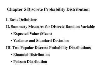
19. Important Distributions 1. Discrete Probability Distribution • Hypergeometric distribution • Binomial distribution • Poisson Distribution 2. Continuous Probability Distribution • Normal distribution • Chi-Square distribution • Student t distribution

20. D Items of Interest N Total # of items n (w/o replacement) x ~Hypergeomitric Hypergeometric Distribution • Suppose that there is a FINITE population consisting of N items. Some number , say D (DN), of these items fall into a class of interest. A random sample of n items is selected from the population without replacement, and the number of items in the sample that fall into the class of interest, say x, is observed.

21. x=0, 1,…,min(n,D) Hypergeometric Distribution • Then x is a Hypergeometric random variable with the probability distribution: • Used as a model when selecting a random sample of n items without replacement from a lot of N items of which D are noncomforming or defective • Excel function: HYPGEOMDIST(x,n,D,N)

22. Example: Special-purpose circuit boards are produced in lots of size N = 20. The boards are accepted in a sample of n = 3 if all are conforming. The entire sample is drawn from the lot at one time and tested. If the lot contains D=3 nonconforming boards, what is the probability of acceptance?

23. Example: A lot of size N = 30 contains five nonconforming units. What is the probability that a sample of five units selected at random contains exactly one nonconforming units? What is the probability that it contains one or more nonconformances?

24. Binomial Distribution • Bernoulli trial: is an experiment with two and ONLY two possible outcomes, either a “success” (1) or a “failure” (0) • Examples of Bernoulli trials • Play slot machine (outcome: win/lose) • Toss coin (outcome: head/tail) • Going to class (outcome: on time/late) • Parts produced by a machine (good/defective) with probability of p with probability of 1 - p

25. Binomial Distribution Binomial Distribution: If n identical (the probability of success on any trial is a constant, p) Bernoulli trials are performed, the number of "success" x in n Bernoulli trials has the Binomial distribution. , and Assumption: (1) Constant probability of success p; (2) Two mutually exclusive outcomes; (3) All trials statistically independent; (4) Number of trials n is known and constant Application: used as a model when sampling from an infinitely large population. The constant prepresents the fraction of defective or nonconforming items in the population Excel Function: BINOMDIST(x,n,p,false) (True:accumulative probability)

27. Estimation of Binomial Distribution Parameter • is the ratio of the observed number of defective or nonconforming items in a sample x to the sample size n • the probability distribution of is obtained from the binomial -> Random number

28. Example: Sixty percent of pulleys are produced using Lathe #1, 40% are produced using Lathe #2. What is the probability that exactly three out of a random sample of four production parts will come from Lathe #1 ?

29. Example: A production process operates with 2% nonconforming output. Every hour a sample of 50 units of product is taken, and the number of nonconforming units counted. If one or more nonconforming units are found, the process is stopped and the quality control technician must search for the cause of nonconforming production. Evaluate this decision rule.

30. Example: A firm claims that 99% of their products meet specifications. To support this claim, an inspector draws a random sample of 20 items and ships the lot if the entire sample is in conformance. Find the probability of committing both of the following errors: (1) Refusing to ship a lot even though 99% of the items are in conformance.(2) Shipping a lot even though only 95% of the items are conforming.

31. Example: A random sample of 100 units is drawn from a production process every half hour. The fraction of nonconforming product manufactured is 0.03. What is the probability that if the fraction nonconforming is actually 0.03?

32. Poisson Distribution Poisson Distribution: the number of random events occur during a specific “time” period with the average occurrence rate  known: • Examples: • A. number of random occurrence per unit of time: number of arrivals to McDonald ’s drive-through window from 12:00~1:00pm • B: number of “defect” per unit of area: number of typographical errors on a page • C: number of “defect” per unit: number of dents on a car • Assumptions: • The average occurrence rate  (per unit) is a known as a constant • Occurrences are equally likely to occur within any unit of time/area • Occurrences are statistically independent Excel Function: POISSON(x,, false) (True: cumulative probability)

34. Example: Arrivals of parts at a repair station are Poisson distributed, with a mean rate of 1.2 per day. What is the probability of no repairs in the next day? What is the probability that today the number of parts requiring repair will exceed the average by more than one standard deviation?

35. Exercises of Discrete Distributions (1) • A production process operates with 2% nonconforming output. Every hour a sample of 50 units of product is taken, and the number of nonconforming units counted as x. • 60% of pulleys are produced using Lathe #1, 40% are produced using Lathe #2. A random sample of four production parts containing x parts coming from Lathe #1. • Circuit boards are produced in lots of size 20. The sample of size 3 is drawn from the lot at one time and tested. The lot contains 3 nonconforming boards and x is the number of nonconforming boards in the sample. • Let x be the number of misprints on one page of a daily newspaper, if the average misprints per page is 2. • 1000 fish in a pond, 100 of them are tagged. x is # of tagged fish among 5 randomly caught fish What is the distribution of x in the following scenarios?

36. Accidents in a building are assumed to occur randomly with an average rate of 36 per year. There will be x accidents in the coming April. • A book of 200 pages with 2 error pages. There are x error pages in a random selection of 10 pages • The probability that a salesman will make a sale on one call is 0.3. Each day, this salesman makes 10 calls. Let x denote the number of sales made in one day. • The average number of flaws per running yard of a certain type of cotton fabric is 0.01. Let x be the number of flaws in a 100-yard roll of this fabric. • The probability that a basketball player will make a free throw is 0.7. Let x denote the number of free throws he will make in a game of seven free throw attempts.

37. f(x) 2 x  Normal Distribution Pr(x+)=68.26% Pr(2x+2)=95.46% Pr(3x+3)=99.73% If x1, x2 are independently normally distributed variables, then y=x1+x2 also follows the normal distribution, i.e. y~N(1+2,12+ 22) The Center Limit Theorem: if x1, x2, …, xnare independent random variables, with mean i and variance i2, and if y=x1+x2+…+xn, then the distribution of z approaches the N(0,1) distribution as n approaches infinite. Excel Function: NORMDIST(x,,,true)

39. Example 3-3

40. Example 3-6: Three shafts are made and assembled in a linkage. The length of each shaft, in centimeters, is distributed as follows: Shaft 1: N ~ (75, 0.09) Shaft 2: N ~ (60, 0.16) Shaft 3: N ~ (25, 0.25) Assume the shafts’ length are independent to each other:(a) What is the distribution of the linkage? (b) What is the probability that the linkage will be longer than 160.5 cm?

42. Chi–Squared Distribution (with degrees of freedom ) y>0 Y follows If x1, x2, …, xn are normally and independently distributed random variables

43. Student t Distribution (with degrees of freedom ) Application: If x and y are independent standard normal and chi-square random variable respectively, thenis distributed as t with k degrees of freedom. Used for testing hypotheses about two population means.

44. F Distribution (with u and v degrees of freedom) If w and y are two independent chi-square random variables with u and v degrees of freedom, respectively, then the ratio is distributed as F with u numerator degrees of freedom and v denominator degrees of freedom. Used for testing hypotheses about two population variances.

46. Useful Results on Mean and Variance If x is a random variable and a is a constant, then E(a+x)=a+E(x) E(a*x)=aE(x) V(a+x)=V(x) V(a*x)=a2V(x) If x1, x2, …, xn are random variables, E(x1+…+xn)=E(x1)+…+E(xn) If they are mutually independent, and a1,…,an are constants V(a1x1+…+ anxn)=a12V(x1)+…+an2V(xn)

47. INTERRELATIONSHIPS BETWEEN DISTRIBUTIONS Hypergeometric, Binomial, Poisson, Normal Hypergeometric finite population if n/N0.1 Sampling without replacement in finite population N: population size n:sample size p=D/N, n The sum of a sequence of n Bernoulli trials in infinite population with probability of success p Binomial if large n, small p <0.1, or large n, large p > 0.9, p’=1-p If np>10 and 0.1 ≤p ≤ 0.9 =np, 2=np(1-p) Number of defects per unit Poisson if 15 = , 2=  Normal

48. Example: An electronic component for a laser range-finder is produced in lots of size N = 25. An acceptance testing procedure is used by the purchaser to protect against lots that contain too many nonconforming components. The procedure consists of selecting five components at random from the lot (without replacement) and testing them. If none of the components is nonconforming, the lot is accepted.a. If the lot contains three nonconforming components, what is the probability of lot acceptance?b. Calculate the desired probability in (a) using the binomial approximation. Is this approximation satisfactory'? Why or why not?c. Suppose the lot size was N=150. Would the binomial approximation be satisfactory in this case?d. Suppose that the purchaser will reject the lot with the decision rule of finding one or more nonconforming components in a sample of size n, and wants the lot to be rejected with probability at least 0.95 if the lot contains five or more nonconforming components. How large should the sample size n be?

50. Example: A textbook has 500 pages on which typographical errors could occur. Suppose that there are exactly 10 such errors randomly located on those pages. Find the probability that a random selection of 50 pages will contain no errors. Find the probability that 50 randomly selected pages will contain at least two errors.