2.1
2.1. Linear Functions and Models. Graphing Discrete Data. We can graph the points and see if they are linear. Enter the data from example 1 into L1 and L2 Stat Edit

2.1
E N D
Presentation Transcript
2.1 Linear Functions and Models
Graphing Discrete Data • We can graph the points and see if they are linear. • Enter the data from example 1 into L1 and L2 • Stat • Edit • Enter the data…if there is already data in your lists you can more the cursor to the very top (on L1) and press clear enter. This will clear the list. • Turn Stat plot on • Press 2nd y= (stat plot) • Select 1 • Select on • Type: first option, this is the scatter plot • Graph the scatter plot • Zoom • Zoomstat – this changes the window to values that are best for your set of data, without us having to pick the best window
Graphing Discrete Data • Check by graphing the equation as well • Put the equation into y1 • Press trace or graph • The line should go through all of the points • When you are done using the stat plot option go to stat plot and choose 4:plots off enter. This will shut off the statplots. • To change your window back to standard –10-10 press zoom, zoom standard
The Regression Line • The Regression Line • Also called the least-squares fit • Approximate model for functions • Uses of the regression line • Finding slope…tells us how the data values are changing. • Analyzing trends • Predicting the future (not always accurate) • Shows linear trend of the data
Linear Regression Line • Enter data into L1 and L2 • Plot the scatter plot • Go to stat • Calc • LinReg(a + bx) • Enter • Enter • a = slope, b = y-intercept • Graph with the points to see how close it is.
Linear Equations • If the equation has a constant rate of change then it is a line. • Linear functions are formulas for graphing straight lines. • Slope intercept form: y = mx + b • Standard form: ax + by = c, a and b are both integers, a>0
Writing equations- given slope and initial value • The initial value is when x = 0, which happens to be the y-intercept (b) • Use y = mx + b • Initial value of 35, slope of ½ • A phone company charges a flat fee of $29.99 plus $0.05 a minute.
Example • A local school is going on a field trip. The cost is $130 for the bus and an additional $2 per child. • Write a formula for the linear function that models the cost for n children. • How much is it for 15 children to attend?
2.2 Equations of Lines
Point-Slope Form • Given point, (a, b), and slope, m, the equation can be found using the formula y – b = m(x – a). This is called the point-slope form of the line.
Examples • Find the equation of the line passing through the given point with the given slope. Write your answer in point slope form. • (6, 12), m = –1/3 • (1, -4), m = 1/3
Examples • Find the equation of the line passing through the given points. Use the first point as (x1,y1) and write your answer in point slope form. • (-2,3), (1,0) • (-1,2), (-2,-3)
Slope-Intercept Form of a Line • Slope Intercept form of a line: • y = mx + b • m = slope • b= y-intercept
Writing equations- given slope and a point • Find the equation of each line in point slope form and in slope-intercept form. • (2,3) m = ½ • (-3, 5) m = 2 • (-8, 7) m = -3/2
Intercepts • Horizontal Intercept- where the line crosses the x axis • This can be found by letting y = 0 • Vertical Intercept- where the line crosses the y axis • This can be found by letting x = 0.
Examples • Locate the x- and y-intercepts on the following lines. • -3x – 5y = 15 • (2/3)y – x = 1
Horizontal and Vertical Lines • An equation of the horizontal line with y-intercept b is y = b. • An equation of the vertical line with x-intercept k is x = k.
Find the equation of the line satisfying the conditions: • Vertical passing through (1.95, 10.7) • Horizontal passing through (1.95, 10.7)
Parallel and Perpendicular Lines • Parallel lines have the same slope. (They are changing at the same rate) • Slopes of perpendicular lines are negative reciprocals of one other. • Ex: ½ and -2; 2/3 and -3/2; -5 and 1/5
For each of the following pairs of lines, determine whether the lines are parallel, perpendicular or neither. a. 3x + 2y = 4 and 6x + 4y = 9 b. 5x – 7y = 3 and 4x – 3y = 8
Examples c. 5x – 7y = 15 and 15y - 21x = 7 d. ax = by = c and akx +aky = d, (a ≠ 0)
Write the Equation Parallel to a given line • 2x – 3y = 9, (-9, 7) • 4x + 5y = 16, (-2, 3)
Write the Equation Perpendicular to a given line • 3x + 4y = 8, (7, 3) • 2x – 8y = 10, (1, 0)
Example • Show that the points (1, 1), (3,4) and (4,-1) from the vertices of a right triangle.
Interpolation • Estimates values that are between two or more known data values. • Extrapolation • Estimates values that are not between two known data values.
Direct Variation • Let x and y denote two quantities. Then y is directly proportional to x, or y varies directly with x, if there exists a nonzero number k such that y = kx. • k is called the constant of proportionality or the constant of variation.
2.3 Linear Equations
Page 118 #18 • Page 118 #20
Page 118 #22 • Page 118 #24
Page 118 #30 • Page 119 #36
Page 119 #60 • Page 119 #64
2.4 Linear Inequalities
A linear inequality in one variable is an inequality that cab be written in the form ax + b >0 where a ≠ 0. (The symbol > can be replaced by <, ≤, or ≥)
Interval Notation • Open interval ( ) • Half-open interval ( ], [ ) • Closed interval [ ] • Infinite intervals
Page 134 #4 • #6 • #8 • #10
Follow the equation rules when solving inequalities. • When you multiply or divide both sides by a negative flip the inequality sign.
Page 134 #14 • Page 135 #18
Page 135 #22 • Page 135 #28