Download
1 / 26
260 likes | 313 Vues
Learn about transfer functions, representation of linear models, definitions, development, examples, and useful conclusions for analysis. Discover how to calculate gains, steady-state responses, model orders, and physical realizability. Explore the simplification and linearization of nonlinear models using Taylor series.

E N D
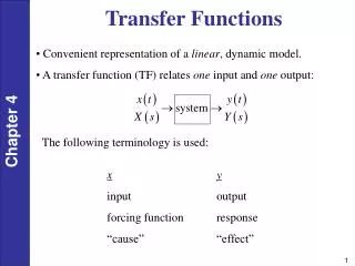
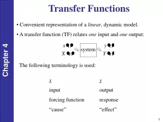
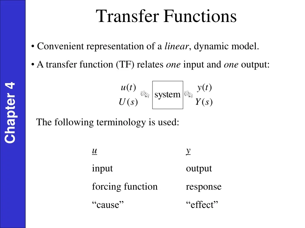
Transfer Functions • Convenient representation of a linear, dynamic model. • A transfer function (TF) relates one input and one output: Chapter 4 The following terminology is used: u input forcing function “cause” y output response “effect”
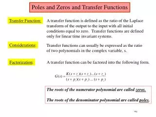
Definition of the transfer function: Let G(s) denote the transfer function between an input, x, and an output, y. Then, by definition where: Chapter 4 Development of Transfer Functions Example: Stirred Tank Heating System
Chapter 4 Figure 2.3 Stirred-tank heating process with constant holdup, V.
Recall the previous dynamic model, assuming constant liquid holdup and flow rates: Suppose the process is at steady state: Chapter 4 Subtract (2) from (2-36):
But, where the “deviation variables” are Chapter 4 TakeLof (4): At the initial steady state, T′(0) = 0.
Rearrange (5) to solve for where Chapter 4
G1 and G2 are transfer functions and independent of the inputs, Q′ and Ti′. Note G1 (process) has gain K and time constant t. G2 (disturbance) has gain=1 and time constant t. gain = G(s=0). Both are first order processes. Chapter 4 If there is no change in inlet temperature (Ti′= 0), then Ti′(s) = 0. System can be forced by a change in either Ti or Q (see Example 4.3).
Conclusions about TFs • 1. Note that (6) shows that the effects of changes in both Q and are additive. This always occurs for linear, dynamic models (like TFs) because the Principle of Superposition is valid. Chapter 4 • The TF model enables us to determine the output response to any change in an input. • Use deviation variables to eliminate initial conditions for TF models.
Example: Stirred Tank Heater No change in Ti′ Step change in Q(t): 1500 cal/sec to 2000 cal/sec Chapter 4 What is T′(t)? From line 13, Table 3.1
Properties of Transfer Function Models • Steady-State Gain • The steady-state of a TF can be used to calculate the steady-state change in an output due to a steady-state change in the input. For example, suppose we know two steady states for an input, u, and an output, y. Then we can calculate the steady-state gain, K, from: Chapter 4 For a linear system, K is a constant. But for a nonlinear system, K will depend on the operating condition
Calculation of K from the TF Model: If a TF model has a steady-state gain, then: • This important result is a consequence of the Final Value Theorem • Note: Some TF models do not have a steady-state gain (e.g., integrating process in Ch. 5) Chapter 4
Order of a TF Model • Consider a general n-th order, linear ODE: Chapter 4 Take L, assuming the initial conditions are all zero. Rearranging gives the TF:
Definition: The order of the TF is defined to be the order of the denominator polynomial. Note: The order of the TF is equal to the order of the ODE. Physical Realizability: Chapter 4 For any physical system, in (4-38). Otherwise, the system response to a step input will be an impulse. This can’t happen. Example:
2nd order process General 2nd order ODE: Laplace Transform: Chapter 4 2 roots : real roots : imaginary roots
Examples 1. (no oscillation) Chapter 4 2. (oscillation)
From Table 3.1, line 17 Chapter 4
Two IMPORTANT properties (L.T.) A. Multiplicative Rule Chapter 4 B. Additive Rule
Example 1: Place sensor for temperature downstream from heated tank (transport lag) Distance L for plug flow, Dead time Chapter 4 V = fluid velocity Tank: Sensor: is very small (neglect) Overall transfer function:
Linearization of Nonlinear Models • Required to derive transfer function. • Good approximation near a given operating point. • Gain, time constants may change with • operating point. • Use 1st order Taylor series. Chapter 4 (4-60) (4-61) Subtract steady-state equation from dynamic equation (4-62)
Example 3: q0: control, qi: disturbance Use L.T. Chapter 4 (deviation variables) suppose q0 is constant pure integrator (ramp) for step change in qi
If q0 is manipulated by a flow control valve, nonlinear element Figure 2.5 Chapter 4 Linear model R: line and valve resistance linear ODE : eq. (4-74)
Perform Taylor series of right hand side Chapter 4
Chapter 4 Next chapter Previous chapter