Dynamic Response of Simple Transfer Functions
460 likes | 759 Vues
Dynamic Response of Simple Transfer Functions. Standard process inputs. Step input Ramp input Rectangular pulse Sinusoidal input Impulse input. Response of 1 st -order process --- Step input. Response of 1 st -order process --- Ramp input. Response of 1 st -order process

Dynamic Response of Simple Transfer Functions
E N D
Presentation Transcript
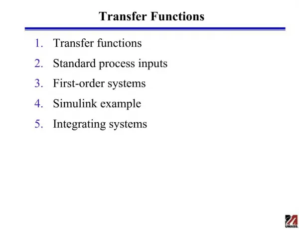
Standard process inputs • Step input • Ramp input • Rectangular pulse • Sinusoidal input • Impulse input
Response of 1st-order process --- Ramp input
Response of 1st-order process ---- Sinusoidal input
Response of 1ST-order process --- Step response with dead time
Over damped process Under damped process
Y(t)/kp t/t
Areaa = m Slope=S y Inflection Point K I3 I2 tm q I1 qS
0.73 y/k t0.73/(t1+t2) 0.5
0.73 y/k 0.5
y/k t/t
Rise time= t0.9-t0.1 b d c a
Overshoot =(y1-yss)/yss b y1 y3 d c yss a y2
Decay ratio=(y3-yss)/(y1-yss ) b y1 y3 yss d c yss a y2
Settling time b y1 y3 yss d c yss a y2 ts
y/k t/t
Dynamic Response Characteristics of More Complicated Process • Pole and zero Effect on dynamic response • Pure time delay: polynomial approximation to • Approximation of higher order transfer functions : Half Rule • Interacting and non-interacting processes
Pole and zero and their effects on dynamic response (continued)
Pole and zero and their effects on dynamic response (continued)
Pole and zero and their effects on dynamic response (continued) See Page 138
Pure time delay y(t) x(t)
Approximation of higher order transfer functions---Half rule • Half of the largest neglected time constant to the existing time delay (if any) • The other half is added to the smallest retained time constant • Time constants smaller than the largest neglected time constant are approximated as time delay by:
Half rule: Examples Neglected time constants: 3, 0.5, -0.1 Approximation:
Half rule: Example 2 Approximation: Neglected time constants: 0.2, 0.05
100oC T 20oC 0% [ T ] 100% T- 20 = 80 x { [T]/100}
Scaling: T- 20 = 80 x { [T]/100} Ts-20 = 80 x { [Ts]/100} G = 80/100 [G] = ST/100 [G] M = Sm/100 [M]
Y(s) M(s) 100% 0%