Development of Transfer Functions in Control Systems
Learn how to create transfer functions for linear dynamic models in Chapter 4. Understand the principles, calculations, and application of transfer functions in practical examples. Gain insights into steady-state gain, physical realizability, and linearization of nonlinear models.

Development of Transfer Functions in Control Systems
E N D
Presentation Transcript
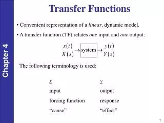
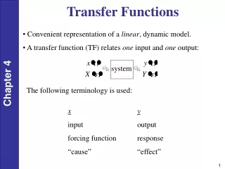
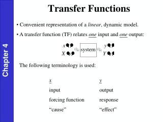
Transfer Functions • Convenient representation of a linear, dynamic model. • A transfer function (TF) relates one input and one output: Chapter 4 The following terminology is used: x input forcing function “cause” y output response “effect”
Development of Transfer Functions Chapter 4 Figure 2.3 Stirred-tank heating process with constant holdup, V.
Recall the previous dynamic model, assuming constant liquid holdup (V) and flow rates (w): Suppose the process is at steady state: Chapter 4 Subtract (2) from (1):
But, where the “deviation variables” are Chapter 4 TakeLof (4): At the initial steady state, T′(0) = 0.
Rearrange (5) to solve for where Chapter 4
Remarks • G1 and G2 are transfer functions and independent of the inputs, Q′ and Ti′. • Both transfer functions are first order. • G1 (process) has gain K and time constant t. • G2 (disturbance) has gain 1 and time constant t. • System can be forced by a change in either Ti or Q. • If there is no change in inlet temperature, then Ti′(t) = 0. Similarly, Q’(t)=0 if there is no change in heat input.
Conclusions about TFs • Use deviation variables to eliminate initial conditions for TF models. • The TF model enables us to determine the output response to any change in an input. • Note that (6) shows that the effects of changes in both Q and Ti are additive. This always occurs for linear, dynamic models (like TFs) because the Principle of Superposition is valid.
Example: Stirred Tank Heater (No change in Ti′) Step change in Q(t): from 1500 cal/sec to 2000 cal/sec Chapter 4 What is T′(t)?
Steady-State Gain The steady-state of a TF can be used to calculate the steady-state change in an output due to a steady-state change in the input. For example, suppose we know two steady states for an input, u, and an output, y. Then we can calculate the steady-state gain, K, from: For a linear system, K is a constant. But for a nonlinear system, K will depend on the operating condition of the initial steady state.
Calculation of Steady-State Gain (K) from the TF Model If a TF model has a steady-state gain, then: • This important result is a consequence of the Final Value Theorem • Note: Some TF models do not have a steady-state gain (e.g., integrating process in Ch. 5)
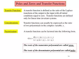
Higher-Order Transfer Functions Consider a general n-th order, linear ODE: Take L, assuming the initial conditions are all zero. Rearranging gives the TF:
Order of Transfer Function • The order of the TF is defined to be the order of the denominator polynomial. • The order of the TF is equal to the order of the ODE.
Physical Realizability • For any physical system, in transfer function. Otherwise, the system response to a step input will be an impulse. This can’t happen. • Example:
2nd-Order Processes The general 2nd order ODE: Laplace Transform: Chapter 4 2 roots : real roots : complexconjugate roots
Examples 1. (no oscillation) Chapter 4 2. (oscillation)
Alternative Solution: From Table 3.1, line 17 Chapter 4
Two IMPORTANT properties of T.F. A. Multiplicative Rule Chapter 4 B. Additive Rule
Example: Place sensor for temperature downstream from heated tank (transport lag) Distance L for plug flow, Dead time Chapter 4 V = fluid velocity Tank: Sensor: is very small (negligible) Overall transfer function:
Linearization of Nonlinear Models • Required to derive transfer function. • Approximation near a given operating point. • Gain, time constants may change with operating point. • Use 1st order Taylor series. Chapter 4 (4-60) (4-61) Subtract steady-state equation from dynamic equation (4-62)
Linear Example pure integrator (ramp) for step change in qi
Nonlinear Example if q0 is manipulated by a flow control valve, nonlinear element