Escaping Local Optima
Escaping Local Optima. Where are we?. Optimization methods. Complete solutions. Partial solutions. Exhaustive search Branch and bound Greedy Best first A* Divide and Conquer Dynamic programming. Exhaustive search Hill climbing. Improved methods based on complete solutions.

Escaping Local Optima
E N D
Presentation Transcript
Where are we? Optimization methods Complete solutions Partial solutions Exhaustive search Branch and bound Greedy Best first A* Divide and Conquer Dynamic programming Exhaustive search Hill climbing
Improved methods based on complete solutions Where are we going? Optimization methods Complete solutions Partial solutions Exhaustive search Branch and bound Greedy Best first A* Divide and Conquer Dynamic programming Exhaustive search Hill climbing
Escaping local optima Many strategies including • Simulated annealing • Tabu search • and many others… some examples -->
(0) Basic Hill climbing determine initial solution s while s is not a local optimum choose s’ in N(s) such that f(s’)>f(s) s = s’ return s
(1) Randomized Hill climbing determine initial solution s; bestS = s while termination condition not satisfied with probability p choose neighbour s’ at random (uniform) else choose s’ with f(s’) > f(s) //climb if possible or s’ with max (f(s’)) over N(s) s = s’; if (f(s) > f(bestS)) bestS = s return bestS
(2) Variable Neighbourhood determine initial solution s i = 1 repeat choose neighbour s’ in Ni(s) with max(f(s’)) if ((f(s’) > f(s)) s = s’ i = 1 // restart in first neighbourhood else i = i+1 // go to next neighbourhood until i > iMax return s
Stochastic local search • many other important algorithms address the problem of avoiding the trap of local optima (possible source of project topics) • M&F focus on two only • simulated annealing • tabu search
Simulated annealing • metaphor: slow cooling of liquid metals to allow crystal structure to align properly • “temperature” T is slowly lowered to reduce random movement of solution s in solution space
Simulated Annealing determine initial solution s; bestS = s T = T0 while termination condition not satisfied choose s’ in N(s) probabilistically if (s’ is “acceptable”) // function of T s = s’ if (f(s) > f(sBest)) bestS = s update T return bestS
determine initial solution s; bestS = s T = T0 while termination condition not satisfied choose s’ in N(s) probabilistically if (s’ is “acceptable”) // function of T s = s’ if (f(s) > f(sBest)) bestS = s update T return bestS Accepting a new solution - acceptance more likely if f(s’) > f(s) - as execution proceeds, probability of acceptance of s’ with f(s’) < f(s) decreases (becomes more like hillclimbing)
the acceptance function T evolves *sometimes p=1 when f(s’)-f(s)> 0
Simulated annealing with SAT algorithm p.123 SA-SAT propositions: P1,… Pn expression: F = D1D2…Dk where clause Di is a disjunction of propositions and negative props e.g., Px ~Py Pz ~Pw fitness function: number of true clauses
Inner iteration assign random truth set TFFT repeat for i=1 to 4 flip truth of prop i FFFT evaluate FTFT decide to keep (or not) FFTT changed value FFTF reduce TFFTT
Tabu search (taboo) always looks for best solution but some choices (neighbours) are ineligible (tabu) ineligibility is based on recent moves: once a neighbour edge is used, it is tabu for a few iterations search does not stop at local optimum
Symmetric TSP example set of 9 cities {A,B,C,D,E,F,G,H,I} neighbour definition based on 2-opt* (27 neighbours) current sequence: B - D - A - I - H - F - E - C - G - B move to 2-opt neighbour B - E - F - H - I - A - D - C - G - B edges B-E and D-C are now tabu i.e., next 2-opt swap cannot involve these edges *example in book uses 2-swap, p 131
TSP example, algorithm p 133 how long will an edge be tabu? 3 iterations how to track and restore eligibility? data structure to store tabu status of 9*8/2 = 36 edges B - D - A - I - H - F- E - C - G - B recency-based memory
procedure tabu search begin tries <- 0 repeat generate a tour count <- 0 repeat identify a set T of 2-opt moves select best admissible move from T make appropriate 2-opt update tabu list and other vars if new tour is best-so-far for a given tries update local best tour information count <- count + 1 until count == ITER tries <- tries + 1 if best-so-far for given tries is best-so-far (for all ‘tries’) update global best information until tries == MAX-TRIES end
applying 2-opt with tabu • from the table, some edges are tabu: B - D - A - I - H - F- E - C - G - B • 2-opt can only consider: • AI and FE • AI and CG • FE and CG
importance of parameters • once algorithm is designed, it must be “tuned” to the problem • selecting fitness function and neighbourhood definition • setting values for parameters • this is usually done experimentally
procedure tabu search begin tries <- 0 repeat generate a tour count <- 0 repeat identify a set T of 2-opt moves select best admissible move from T make appropriate 2-opt update tabu listand other vars if new tour is best-so-far for a given tries update local best tour information count <- count + 1 until count == ITER tries <- tries + 1 if best-so-far for given tour is best-so-far for all tries update global best information until tries == MAX-TRIES end