Download
1 / 12
120 likes | 290 Vues
Parameter optimization in an atmospheric GCM using Simultaneous Perturbation Stochastic Approximation (SPSA) Reema Agarwal (reema.agarwal@zmaw.de) , Armin Köhl , Detlef Stammer Centrum für Erdsystemforschung und Nachhaltigkeit (CEN) Universität Hamburg, Hamburg , Germany.

E N D
Parameter optimization in an atmospheric GCM using Simultaneous Perturbation Stochastic Approximation (SPSA) Reema Agarwal (reema.agarwal@zmaw.de), Armin Köhl, Detlef Stammer Centrum fürErdsystemforschung und Nachhaltigkeit (CEN) Universität Hamburg, Hamburg, Germany The research leading to these results has received funding from NACLIM, a project of the European Union 7th Framework Programme (FP7 2007-2013) under grant agreement n.308299
Objective • Automatized model tuning to reduce model errors • To improve AGCM through parameter optimization Model used and Control parameters • AGCM Planet Simulator (Plasim, Fraedrich et al. 2005) with spectral resolution T21 and 10 vertical sigma levels • 14 control parameters used in the parameterization of long wave-short wave radiation, cloud parameters; vertical diffusion time scales are chosen
Planet Simulator Plasim • Plasim is part of the coupled climate model CESAM(CEN Earth System Assimilation Model http://www.cen.uni-hamburg.de/CESAM-CE.2376.0.html) • Simplified parameterizations are included for boundary layer fluxes and diffusion, radiation and moist processes with interactive clouds. • Land and soil temperatures, soil hydrology and river runoff • Not enabledarereducedmodelsfor • land-vegetation • sea ice model • mixed layer ocean model
SPSA “Simultaneous Perturbation” and gradient approximation (Spall et al. 1987)
Data sets for optimization • Pseudo data (produced by model itself in a run with default values of all control parameters ) • ERA-Interim Reanalysis data from fields of temperature (all • 10 levels), total precipitation and net heat flux is used • Annual means • Optimization of an already hand tuned model Sensitivity experiments • Over long periods of time the nonlinear dynamics of the model is transformed into stochastic perturbations of cost function • Range of cost function values larger than zero if parameter perturbations are not precisely zero
Identical twin experiments • A model run of 1-year was performed with a set of randomly chosen values of 14 parameters • The cost function reaches the acceptable minimum value of ~20 as shown in the sensitivity experiments • Only those 8 of the 14 parameters could be retrieved for which the costfunction is not flat Cost function vs. iteration number for selected 14 parameters in the identical twin experiment. Cost function is computed for a period of 1 year model integration.
Experiments with ERA-Interim • To test the robustness of technique ,3 different experiments were performed • The initial value of each control parameter is increased by 0%, 60% and 100% • Due to the flat minima with the presence of “noise”, different sets of parameters are obtained from the 3 experiments and their relative error remained almost constant
Results continued RMSE of individual contributions in original and optimized model states. The reduction is ~20%, 5%, 11% and 18% for Temperature, precipitation, net heat flux and surface temperature RMSE of global mean Temperature between ERA-interim and Original and optimized model runs. Y axis denotes height of the atmosphere represented as sigma levels with model level 10 corresponding to bottom and model level 1 corresponding to the top of the atmosphere
Results continued Near surface Temperature(K) Annual root mean squared differences (RMSD) of ERA-interim with Original (top panels) and Optimized (bottom panels) model variable
Results continued Annual root mean squared differences (RMSD) of ERA-interim with Original (top panels) and Optimized (bottom panels) model variable
Conclusions • SPSA is easy to implement and computationally efficient • SPSA can handle chaotic models • For an already hand tuned model, the overall reduction in RMSE is ~ 16% with respect to ERA-interim observations while surface temperatures shows improvement up to 18%