Systematic Errors and Sample Preparation for X-Ray Powder Diffraction
Systematic Errors and Sample Preparation for X-Ray Powder Diffraction. Jim Connolly EPS400-001, Spring 2010. Introduction. Most systematic errors in diffraction experiments are related to the characteristics, preparation and placement of the specimen. Today we will:

Systematic Errors and Sample Preparation for X-Ray Powder Diffraction
E N D
Presentation Transcript
Systematic Errors and Sample Preparation for X-Ray Powder Diffraction Jim Connolly EPS400-001, Spring 2010
Introduction • Most systematic errors in diffraction experiments are related to the characteristics, preparation and placement of the specimen. Today we will: • Differentiate and define those errors • Present preparation techniques to minimize those errors • Discuss different types of sample mounting strategies and trade-offs of various methods • Always remember the distinction between sample and specimen • Footnote question: What is the difference between a random and systematic error?
Goals of Specimen Preparation • Overall Rule: The time and effort put into specimen preparation should not be more than is required by the experiment objective • Basic information in the diffraction pattern: • The position of the diffraction peaks • The peak intensities, and shape of peaks • The intensity distribution as a function of diffraction angle • The utility of this information depends on both the experiment parameters and the sample preparation • Communicate with your “client” about the objectives of your experiment • Design your experiment to achieve those objectives
Specimens and Experimental Errors • Axial Divergence: The X-ray beam diverges out of the plane of the focusing circle • Flat Specimen Error: The specimen is flat, and does not follow the curvature of the focusing circle. • Compositional Variations between Sample and Specimen • Specimen Displacement: Position of the sample mount causes deviation of the focusing circle • Specimen Transparency: Beam penetration into a “thick” specimen changes diffraction geometry • Specimen Thickness: Trade-offs between accuracy of peak positions and intensities • Particle Inhomogeneity: Can significantly alter diffraction intensities • Preferred Orientation: Can produce large variations in intensity and limit the peaks seen.
Beam Path from Source to Detector Path from X-ray source to detector is shown at right Beam path: • From horizontal source F to • vertical soller slits SS1 to • Divergence slit D5 • Specimen S (A=center of diffractometer circle) to • Receiving Scatter slit RS to • Receiving soller slits SS2 to • scatter slit SS to • Monochromator and Detector (not in picture)
Axial Divergence • Detector sees the arc of the Debye ring not just the diffractions along the 2D diffractometer circle • Leads to a notable peak asymmetry, particularly pronounced at low 2θ • Axial Divergence error for Silver Behenate is shown at right • Can be minimized by closely spaced soller slits (at the cost of reduced intensity)
Flat Specimen Error • The extreme edges of the specimen lie on another focusing circle (rf’) which results in the overall diffracted intensity being skewed to a lower value of 2. • This is related to the divergence of the incident beam by the equation below where is the angular aperture of divergence slit in degrees The table at right shows specimen irradiation lengths (in mm) for a diffractometer of a particular radius (not ours)
Differences between Sample and Specimen • Grinding Effects • Problem: Excessive percussive grinding produces extremely small particle size peak broadening • Remedy: Be careful (or use non-percussive grinding techniques) • Irradiation Effects • Interaction with beam changes specimen • Rare in inorganics; significant issue in organics and phases with poorly-bound H2O • Environmental Effects • Strain effects in materials at elevated temperature • Chemical reactivity of specimen • Sensitivity to water, air or other solvents • Usually reversible, sometimes not • Systematically used as a tool in clay analysis
Specimen Displacement • Cause: Specimen is higher or lower than it should be (i.e., not at center of diffractometer circle or tangent to focusing circle) • Effect: 2θ error defined by the following equation: (R is the radius of the diffractometer circle; s is the deviation from the correct position on the focusing circle measured as the difference between r and r’) • Can be a significant cause of errors in 2θ • More pronounced at low θvalues (cosine function) • Can produce asymmetric peak broadening at low angles (resembling axial divergence) • 2θcan be as much as 0.01º for each 15m of displacement at low angles • Can be caused by poor diffractometer alignment
Specimen Transparency • Caused by diffraction occurring at depth within a thick specimen • Results in 2θ related to effective penetration depth of the specimen • The error is defined: • is dependent on mass and the x-ray wavelength • For SiO2 and CuK, = 97.6/cm, or approx. 100/cm. Thus t0.5 thus is about 0.01 cm or 100 m. • For high-density, high / materials (metals, alloys), t0.5 will be on the order of 10 m • For low-density organics, t0.5 will be on the order of 1,000 m, and a thick sample will induce very significant displacement errors • Loose packing of powders can add reduce density and thus increase t0.5 where is the linear attenuation (a.k.a. linear absorption) coefficient for the x-ray wavelength, R is the radius of the diffractometer circle and 2 is in radians Defines the working depth
Specimen Thickness Bottom line for specimens is: • Thin specimens • Yield the best angular measurements (i.e. most accurate peak positions) • Do not yield accurate intensity measurements (because of bad particle statistics) • Tend to be more susceptible to preferred orientation effects • Thick specimens • Can yield good intensity measurements (better particle statistics, less susceptible to preferred orientation) • Susceptible to angular measurement errors
Sample Inhomogeneity • Multi-phase samples may be inhomogeneous • In example at right chalcopyrite CuFeS2 (A) partially oxidized to cuprospinel CuFe2O4 (C) • A and C have different mass attenuation coefficients (143.2 and116.1, respectively) • The result will be diffraction intensities from the two phases that are not directly proportional to the amounts of the phases present • This effect is called the absorption effect or the particle inhomogeneity effect.
Preferred Orientation • Preferred Orientation (lack of random orientation in the powder) is usually the dominant cause of intensity variations in a diffraction pattern. • Effect is most pronounced for crystals with anisotropic shapes (or habits) • This significantly affects the diffracted intensities from the specimen.
Preferred Orientation • Occurs as a consequence of the “spotty” nature of diffraction in a non-random specimen • The effect is that the Debye ring is uneven in intensity
Preferred Orientation • How the preferred orientation is manifest in the diffraction pattern varies with the material • Clay minerals have a platy habit and will orient perpendicular to (00l). • Equant cubes (NaCl) orient parallel to their cubic crystal faces • Bladed (most pyroxenes and amphiboles) or fibrous (most asbestos minerals and some zeolites) materials orient parallel to their elongation direction • Some engineered polymers use preferred orientation for specialized qualities • Severe preferred orientation in a specimen will result in “invisible” diffraction peaks • In most specimens, all of the diffraction peaks will be seen but their relative intensities will differ from the “ideal” pattern. • Careful specimen preparation can minimize the effect • Whole-pattern refinements can use preferred orientation as another parameter to be fit to the data
Particle Statistics • Quantitative (and semi-quantitative) X-ray powder diffraction is based on the principle that quantities are proportional to intensity. • Accurate intensities require: • Random orientation of crystallites in the specimen • Sufficient number of particles for good crystallite statistics Note: Particle size is frequently (erroneously) equated with crystallite size • At right is a schematic pole plot of diffractions from two powder specimens on a sphere • A random pattern indicates a random orientation
A particle statistics exercise • It is instructive to understand how crystallite statistics will quantitatively affect intensity, i.e., what size particles are required to achieve a repeatability in intensity measurements? • Assume a powdered quartz (SiO2) specimen: • Volume = (area of beam) x (2x half-depth of penetration) • Assume area = 1cm x 1cm = 100mm2 • t½ = 1/, where = linear absorption coefficient • SiO2 = 97.6 /cm or ~100 /cm = 10 /mm • V = (100) (2) / 10 mm3 • Thus Volume = 20 mm3 • Estimate number of particles at different particle sizes:
Particle Statistics Exercise (cont.) • Equal distribution on a unit sphere (area = 4 steradians) yields a radiating sheaf of pole vectors • Calculating angular distribution on the sphere:
Particle Statistics Exercise (cont.) • Geometry of diffraction of a single particle: • R is the diffractometer radius (a range is shown), F the focal length of the anode (a characteristic of the x-ray tube), and the angular divergence as shown. In the above example, L (= 0.5 mm) is the length of source visible to the target. • NP (number of diffracting particles) = (area on unit sphere corresponding to divergence) / (area on unit sphere per particle) = AD/AP
Particle Statistics Exercise (cont.) = 2.5 x 10⁻⁴ • To determine AD requires relating effective source area, FxL, to area on a unit sphere: • Calculating AD/AP yields the number of particles diffracting in any given unit area for our three particle sizes: Conclusion: The standard uncertainty in Poisson statistics is proportional to n½, where n is the number of particles. To achieve a relative error of < 1%, we need 2.3 = 2.3 n½ / n < 1%. This requires n > 52, 900 particles! Thus not even 1 m particles will succeed in achieving ±1% accuracy in intensity. The Bottom Line: Easily achievable particle sizes will not routinely yield high-precision, repeatable intensity measurements.
Enough of this Particle Statistics Stuff • Other Factors can degrade or improve intensity accuracy: • Concentration: mixed phase specimens reduce particles of a given phase in a unit area, increasing error • Reflection multiplicity:Multiplicity in higher symmetry crystal structures give more diffraction per unit cell, improving statistics • Specimen thickness: may improve diffraction volume, limited by maximum penetration depth • Peak width (crystallite size): polycrystalline particles with random orientation can greatly improve statistics, but extremely small size will result in peak broadening. • Specimen rotation/rocking: helps to get more particles in the beam. Rocking combined with rotation is best. Ultimately, quantitative analysis based on peak intensities cannot reliably achieve ±1% accuracy even under the most favorable specimen conditions of randomly oriented 1m particles
From Sample to Specimen From rock to powder • Bico Jaw Crusher * (Loc. 1) • Plattner Steel Mortar & Pestle (Loc. 2) • Spex Shatterbox * (Loc. 2) • Mortar & Pestle (Loc. 2 & 3) • Retch-Brinkman Grinder * (Loc. 3) • Sieves for sizing (Loc. 2) • * Manual for use available on class web page • Equipment Locations: • 1 – Northrop Hall Rm 110 • 2 – Geochem Lab, Northrop Hall Rm 213 (see Dr. Mehdi-Ali) • 3 – XRD Lab, Northrop Hall Rm B-25
Various Mortars and Pestles “Diamonite” synthetic alumina Natural Agate
Retch Brinkman Grinder Pestle Motor Pestle Up- Down Pestle Mortar Speed Adjustments
To sieve or not to sieve . . . • Sieves can be metal, teflon or other synthetic • Theoretically 10 m particles may be passed (practically, it doesn’t work) • Because of static forces, 325 mesh is smallest for routine use though 400 and 600 may be used with a lot of effort
Specimen Mounts • How your specimen is mounted should be determined by the requirements of your experiment – i.e., don’t do more or less than is necessary • Know the characteristics of your holder – always run your mount without any specimen to know your baseline “background” conditions Mount Types: • Thin Mounts (best for accurate angular measurements) • Slurry mounts (on any flat substrate) • Double-stick tape • Petroleum jelly “emulsion” • Volume or “Bulk” Mounts (best for accurate intensity measurements) • Side-drift mounts • Top-load mounts • Thin-film mounts • Back-pack mounts • Zero-background (off-axis quartz plate) mounts
Special techniques to reduce preferred orientation • Aerosol Spray Drying using Clear Acrylic Lacquer(procedure outlined in class notes) • Aqueous Spray Drying in a Heated Chamber(details at http://www.macaulay.ac.uk/spraydrykit/index.html)
Coming Attractions: • After Spring Break on Mar 24: In-Class Exam: • Open-book • Start Promptly at 3:00 PM; do not be late • Must complete exam in 1 hour • Written short-answer format • All reference materials okay • Texts will be available for reference • Includes everything through last week (Weeks 1 thru 6) • Emphasis on demonstrating your understanding of material • Followed by: Tour of the XRD Lab • Layout, location of all equipment and computers • Introduction to MDI DataScan program and scheduling of hands-on lab training • Radiation safety exam should be completed before class