Lecture 2 Standardization, Normal distribution, Stem-leaf, histogram
Lecture 2 Standardization, Normal distribution, Stem-leaf, histogram. Standardization is a re-scaling technique, useful for conveying information about the relative standing of any number of interest with respect to the whole distribution Normal distribution : ideal bell shape curve

Lecture 2 Standardization, Normal distribution, Stem-leaf, histogram
E N D
Presentation Transcript
Lecture 2 Standardization, Normal distribution, Stem-leaf, histogram • Standardization is a re-scaling technique, useful for conveying information about the relative standing of any number of interest with respect to the whole distribution • Normal distribution : ideal bell shape curve • Stem-leaf, histogram: empirical STAT 13 -Lecture 2
Measure of dispersion • Maximum - minimum=range • Average distance from average • Average distance from median • Interquartile range= third quartile - first quartile • Standard deviation = square root of ‘average’ squared distance from mean (NOTE: n-1) • The most popular one is standard deviation (SD) • Why range is not popular? • Only two numbers are involved : regardless of what happen between. • Tends to get bigger and bigger as more data arrive STAT 13 -Lecture 2
Why not use average distance from mean? center point= C Ans: the center point C that minimizes the average distance is not mean median Mean=3.7 1.0 2.0 What is it? 2.5 3.0 3.5 4.0 5.5 Ans : median Average dist from median= (1.0+2+0.5+0.5+0)/5=(3.0+1.0+0)/5=5/5 Average dist from mean= (3.0+1.0+**)/5; where **= length of STAT 13 -Lecture 2
Mean or Median • Median is insensitive to outliers. Why not use median all the time? • Hard to manipulate mathematically • Median price of this week (gas) is $1.80 • Last week : $2.0 • What is the median price for last 14 days? • Hard! How about if last week’s median is $1.80 • Still hard. • The answer : anything is possible! Give Examples. • Median minimizes average of absolute distances. STAT 13 -Lecture 2
Mean is still the more popular measure for the location of “center” of data points • What does it minimize? • It minimizes the average of squared distance • The average squared distance from mean is called variance • The squared root of variance is called standard deviation • How about the “n-1” (instead of n, when averaging the squared distance), a big deal ? Why? STAT 13 -Lecture 2
Yes, at least at the conceptual level If n is large, it does not matter to use n or n-1 • Population : the collection of all data that you imagine to have (It can be really there, but most often this is just an ideal world) • Sample : the data you have now • ALL vs. AML example • =====well-trained statistician++++ • Use sample estimates to make inference on population parameters; need sample size adjustment • (will talk about this more later) Sample mean = sum divided by ??? n or n-1? STAT 13 -Lecture 2
One standard deviation within the mean covers about 68 percent of data points • Two standard deviation within the mean cover about 95 percent of data points • The rule is derived under “normal curve” • Examples for how to use normal table. Course scores STAT 13 -Lecture 2
A long list of values from an ideal population Density curve represents the distribution in a way that High value = dense Low value=sparse 75 grade 60 90 mean 0 1 -1 SD=15 • Find mean and Set mean to 0; apply formula to find height of curve • 2. Find SD and set one SD above mean to 1. • 3. Set one SD below mean to -1 STAT 13 -Lecture 2
Normal distribution When does it make sense? Symmetric; one mode • How to draw the curve? • Step 1 : standardization: change from original scaling to standard deviation scaling using the formula z= (x minus mean) divided by SD • Step 2 : the curve has the math form of 1 z2 e 2 2p STAT 13 -Lecture 2
Use normal table • For negative z, page • For positive z, page • Q: suppose your score is 85, What percentage of students score lower than you? • Step 1 : standardization (ask how many SD above or below mean your score is) • answer : z= (85-75)/15=.666 • Look up for z=.66; look up for z=.67; any reasonable value between the two is fine • (to be continued) STAT 13 -Lecture 2
Step by Step illustration for finding median through Stem-leaf plot • (bring final scores for in class demo) • Find Interquartile range • Guess the mean , SD • From Stem-leaf to Histogram • Three types of histograms (equal intervals recommended) STAT 13 -Lecture 2
Homework 1 assigned (due Wed. 2nd week) • Reading mean and median from histogram • Symmetric versus asymmetric plot. • Normal distribution STAT 13 -Lecture 2
From stem-leaf to histogram • Using drug response data • NOT all bar charts are histograms!!! • NCBI’s COMPARE • Histograms have to do with “frequencies” STAT 13 -Lecture 2