Normal Distribution
Normal Distribution. The Bell Curve. Questions. What are the parameters that drive the normal distribution? What does each control? Draw a picture to illustrate. Identify proportions of the normal, e.g., what percent falls above the mean? Between 1 and 2 SDs above the mean?


Normal Distribution
E N D
Presentation Transcript
Normal Distribution The Bell Curve
Questions • What are the parameters that drive the normal distribution? What does each control? Draw a picture to illustrate. • Identify proportions of the normal, e.g., what percent falls above the mean? Between 1 and 2 SDs above the mean? • What is the central limit theorem? • Why is the number 1.96 a big deal? • Describe the standard error of the mean when samples are drawn from a normal distribution.
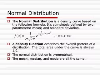
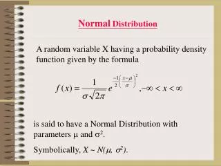
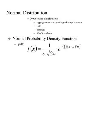
Function • The Normal is a theoretical distribution specified by its two parameters. • It is unimodal and symmetrical. The mode, median and mean are all just in the middle.
Function (2) • There are only 2 variables that determine the curve, the mean and the variance. The rest are constants. • 2 is 2. Pi is about 3.14, and e is the natural exponent (a number between 2 and 3). • In z scores (M=0, SD=1), the equation becomes: (Negative exponent means that big |z| values give small function values in the tails.)
Areas and Probabilities • Cumulative probability:
Areas and Probabilities (2) • Probability of an Interval
Areas and Probabilities (3) • Hays Table 1 shows cumulative normal probabilities. Some selected entries: About 54 % of scores fall below z of .1. About 46 % of scores fall below a z of -.1 (1-.54 = .46). About 14% of scores fall between z of 1 and 2 (.98-.84).
Areas and Probabilities (3) • Using the unit normal (z), we can find areas and probabilities for any normal distribution. • Suppose X=120, M=100, SD=10. Then z=(120-100)/10 = 2. About 98 % of cases fall below a score of 120 if the distribution is normal. In the normal, most (95%) are within 2 SD of the mean. Nearly everybody (99%) is within 3 SD of the mean.
Review • What are the parameters that drive the normal distribution? What does each control? Draw a picture to illustrate. • Identify proportions of the normal, e.g., what percent falls below a z of .4? What part falls below a z of –1?
Importance of the Normal • Errors of measures, perceptions, predictions (residuals, etc.) X = T+e (true score theory) • Distributions of scores (e.g., height) • Math implications (e.g., inferences re variance) • Central Limit Theorem • 1. Sampling distribution of means becomes normal as N increases, regardless of shape of original distribution. • 2. Binomial becomes normal as N increases.
Properties of the Normal • If a distribution is normal, the sampling distribution of the mean is normal regardless of N. • If a distribution is normal, the sampling distributions of the mean and variance are independent.
Confidence Intervals for the Mean • Over samples of size N, the probability is .95 for • Similarly for sample values of the mean, the probability is .95 that • The population mean is likely to be within 2 standard errors of the sample mean. • Can use the Normal to create any size confidence interval (85, 99, etc.)
Size of the Confidence Interval • The size of the confidence interval depends on desired certainty (e.g., 95 vs 99 pct) and the size of std error of mean ( ). • Std err of mean is controlled by population SD and sample size. Can control sample size. • SD 10. If N=25 then SEM = 2 and CI width is about 8. If N=100, then SEM = 1 and CI width is about 4. CI shrinks as N increases. As N gets large, decreasing change in CI because of square root. Less bang for buck as N gets big.
Review • What is the central limit theorem? • Why is the number 1.96 a big deal? • Describe the sampling distribution of the mean when samples are drawn from a normal distribution. • Assume that scores on a curiosity scale are normally distributed. If the sample mean is 50 based on 100 people and the population SD is 10, find an approx 99 pct CI for the population mean.
Computer Exercise • Get data from class (e.g., height in inches) • Compute mean, SD, StErr of Mean in Excel • Compute same in SAS PROC UNIVARIATE • Show plots (stem-leaf & Boxplot) • Show test of normality