Normal Distribution
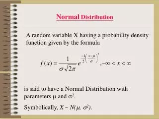
Normal Distribution. The Normal Distribution is a density curve based on the following formula. It’s completely defined by two parameters: mean; and standard deviation. A density function describes the overall pattern of a distribution. The total area under the curve is always 1.0.

Normal Distribution
E N D
Presentation Transcript
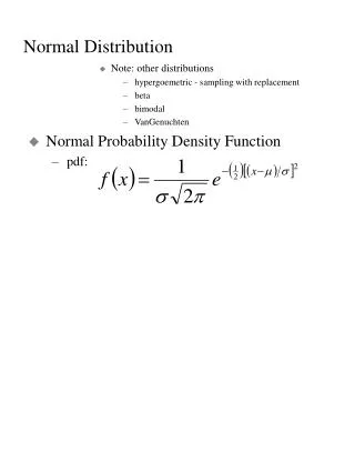
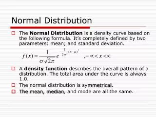
Normal Distribution • The Normal Distribution is a density curve based on the following formula. It’s completely defined by two parameters: mean; and standard deviation. • A density function describes the overall pattern of a distribution. The total area under the curve is always 1.0. • Thenormal distribution is symmetrical. • Themean, median, and mode are all the same.
Normal Distribution If we know µ and σ, we know every thing about the normal distribution. Total area under the curve is 1 σ 2σ µ
Normal Distribution The 68-95-99.7 Rule In the normal distribution with mean µ and standard deviation σ: 68% of the observations fall within σ of the mean µ. 95% of the observations fall within 2σ of the mean µ. 99.7% of the observations fall within 3σ of the mean µ. σ σ 3σ 2σ 2σ 3σ
Normal Density Plot A sample of 100 observations from a normal distribution with mean 0 and standard deviation 1. 68% 95%
Normal Distribution • Standardizing and z-Scores If x is an observation from a distribution that has mean µ and standard deviation σ, the standardized value of x is, A standardized value is often called a z-score. If x is a normal variable with mean µ and standard deviation σ, then z is a standard normal variable with mean 0 and standard deviation 1.
Normal Distribution • Let x1, x2, …., xn be n random variables each with mean µ and standard deviation σ, then sum of them ∑xi be also a normal with mean nµ and standard deviation σ√n. The distribution of mean is also a normal with mean µ and standard deviation σ/√n. • The standardized score of the mean is, The mean of this standardized random variable is 0 and standard deviation is 1.
Assessing the normality of data • Most statistical methods assume that data are from a normal population. So it’s important to test the normality of the data. • Normal quantile plots If the points on a normal quantile plot lie close to diagonal line, the plot indicates that the data are normal. Otherwise, it indicates departure from normality. Points far away from the overall pattern indicates outliers. Minor wiggles can be overlooked. We will see normal quantile plots in next two slides. • Shapiro-Wilk W statistics, Kolmogorov-Smirnov (K-S) tests etc are being used for testing normality of the data. • To perform a K-S Test for Normality in SPSS, Analyze> Nonparametric Tests > 1 Sample K-S. Choose OK after selecting variable (s). • To perform Shapiro-Wilk test of normality in R use the following: >x<- c(12, 14, 13, 11, 16, 18) for inputting data >shapiro.test(x)
Normal quantile plot q-q plot of 100 sample observations from a normal distribution with mean 0 and standard deviation 1
Normal quantile plot This plot shows a minor deviation from the linear diagonal line. We can ignore this minor wiggles and still can assume that the data are from a normal distribution.
Population and Sample • Population: The entire collection of individuals or measurements about which information is desired e.g. If want to know the average height of 5-year old children in USA, then all 5-year old children in USA is our population. • Sample: A subset of the population selected for study. • Methods of sampling: Random sampling, stratified sampling, systematic sampling, cluster sampling, multistage sampling, area sampling, qoata sampling etc. We will discuss only random sampling. • Random Sample: A simple random sample of size n from a population is a subset of n elements from that population where the subset is chosen in such a way that every possible unit of population has the same chance of being selected. • Example: Consider a population of 5 numbers (1, 2, 3, 4, 5). How many random samples (without replacement) of size 2 can we draw from this population ? (1,2), (1,3), (1, 4), (1, 5), (2, 3), (2, 4), (2, 5), (3,4), (3,5), (4,5)
Population and Sample • Why do we need randomness in sampling? It reduces the possibility of subjective and other biases. Mean and variance of a random sample is an unbiased estimate of the population mean and variance respectively. • Population mean of the five numbers in previous slide is 3. Averages of 10 samples of sizes 2 are 1.5, 2, 2.5, 3, 2.5, 3, 3.5, 3.5, 4, 4.5. Mean of this 10 averages (1.5 +2 + 2.5 + 3 + 2.5 + 3+ 3.5+ 3.5+ 4+ 4.5)/10 =3 which is the same as the population mean.
Parameter and Statistic • Parameter: Any statistical characteristic of a population. Population mean, population median, population standard deviation are examples of parameters. • Statistic: Any statistical characteristic of a sample used as an estimate of population parameter such as sample mean, sample median, sample standard deviation etc. • Statistical Issue: Describing population through census or making inference from sample by estimating the value of the parameter using statistic.
Census and Inference • Census: Complete enumeration of population units. • Statistical Inference: We sample the population (in a manner to ensure that the sample correctly represents the population) and then take measurements on our sample and infer (or generalize) back to the population. Example: We may want to know the average height of all adults (over 18 years old) in the U.S. Our population is then all adults over 18 years of age. If we were to census, we would measure every adult and then compute the average. By using statistics, we can take a random sample of adults over 18 years of age, measure their average height, and then infer that the average height of the total population is ``close to'' the average height of our sample.
Univariate, Bivariate, and Multivariate Data • Depending on how many variables we are measuring on the individuals or objects in our sample, we will have one of the three following types of data sets • Univariate: Measurements made on only one variable per observation. • Bivariate: Measurements made on two variables per observation. • Multivariate: Measurements made on more than two variables per observation.
Proportion • Proportion: In many cases, it is appropriate to summarize a group of independent observations by the number of observations in the group that represent one of two outcomes. • Consider a variable X with two outcomes 1 and 0 for happening and not happening of some events correspondingly. Let p be the probability that the event happens then p=Prob(X=1). • Suppose, we want to estimate of the proportion of the Patients coming to duPont having some particular disease. To estimate this proportion (population), we need to take a sample of size n and examine if the patient is bearing that particular disease. Then the estimated proportion is,
Proportion • For large n, the sampling distribution of is approximately normal with mean P (Population Proportion) and the standard deviation • If probability of happening one event is p, then probability of not happening of the same event is 1-p and total probability is 1. • What is the difference between proportion and a sample mean? If X takes two values 0 or 1 and p is the proportion of happening an event (X=1) then the sample proportion is the same as the sample mean. For example, the mean of the following data 1,0,1,1,0 is (1+0+1+1+0)/5 = 3/5 and the proportion is also the 3/5.
Binomial Distribution • Let us consider an experiment with two outcomes success (S) and failure (F) for each subject and the experiment be done for n subjects. One of the possible sequences of S and F can be arranged as follows- SSFSFFFSSFS……F where there are x success out of n trials. Then the probability distribution of x can written as
Binomial Distribution • The mean and variance of x are np and np(1-p). • If p=1/2, then Binomial distribution is symmetric.
Test of hypothesis • A statistical hypothesis is some statement or assertion about the population distribution or population parameter which we want to verify on the basis of information available from a sample. • Test of hypothesis is a two-action decision problem after the sample values have been obtained, the two actions being the acceptance or rejection of the hypothesis under consideration. • Null Hypothesis: The statement is being tested in a test of significance. Usually the null hypothesis is a statement of “no effect” or “no difference”. That is, a statement without any kind of motivation due to any reason. H0 is the abbreviated form of null hypothesis. • Alternative Hypothesis: Complement of null hypothesis. Ha is the abbreviated form of alternative hypothesis.
Test of hypothesis • Test statistic: The statistic is used to test the significance of a hypothesis. • Two types of errors: Type I error and Type II error. • Type I error (α): Probability of rejecting H0 when it is true (Ha is false). • Type II error (β): Probability of rejecting Ha when it is true. Truth about the population H0 true Ha true Decision Based on sample Reject H0 Accept H0
Test of hypothesis • Our aim is to make inference controlling both type I and type II errors. But the reduction in one results in an increase in the other and the consequence of type I error seems to be more severe than that of type II error. That’s why, we choose a test that minimizes type II error (maximize the power of the test) keeping type I error at a fixed low level. • Level of Significance: The probability of type I error is known as the level of significance. • Power (1-β): The probability of rejecting H0 when alternative hypothesis is true at a fixed level of significance (α ). Power of a test is a function of sample size and the parameter of interest. We calculate power for a particular value of the parameter in alternative hypothesis. Increasing sample size increases power of a test. • Increasing Power: If power is too small than we can do the followings to increase power: • Increase the sample size • Increase the significance level (α ) • Reduce the variability
Test of hypothesis • P-value: The probability, assuming H0 is true, that the test statistic would take a value as extreme or more extreme than that actually observed is called the P-value of the test. The smaller the P-value, the stronger the evidence against H0 provided by the data. • Statistical Significance: If the P-value is small or smaller than α, we say that the test is statistically significant at level α. A result is statistically significant if it is unlikely to happen by chance.
Point estimation and Confidence Interval • Two types of parameter estimation: • Point Estimation: A single value calculated from sample data, that estimates the parameter. Unbiasedness, consistency, efficiency, and sufficiency are some of the criteria that should be satisfied by a good estimator. The sample mean is a point estimate of the population mean. • Interval Estimation: A range calculated from sample data along with a confidence level that a population parameter lie between the range is called interval estimate of the parameter. • Confidence Interval: An interval computed from sample data containing the true value of the parameter with a certain level of confidence. With a 95% confidence interval of a mean we mean, 95% of all samples of the same size will contain the true population mean. A confidence interval for mean can be written as follows
Confidence Interval • Confidence Interval = Point Estimate ± Margin of error • Margin of error: The amount of allowed sampling error. • 95% Confidence Interval for mean= Sample mean ± ((z97.5σ/ √n ) or ( t97.5, (n-1)s/ √n)) where s and σ are the sample and population standard deviations correspondingly.
Sampling Distribution • Standard Error: Standard deviation of a statistic. Let x1, x2, …xn be a sample of size n. Then the standard deviation of the sample mean is a standard error. It is written as σ/√n and s/√n termed as estimated standard error of sample mean. • Sampling distribution: The distribution of a statistic. • Commonly used statistic: Z-statistic, t-statistic, chi-square statistic, F-statistic are some of the commonly used statistics.
Z-Score • Z-score: the statistic is distributed as standard normal with mean 0 and standard deviation 1. • Assumptions: Sample is large and the population standard deviation is known. • Applications: • 1. Test of hypothesis of a single sample mean • 2. Comparing means of two groups or populations.
Power Calculation and Sample Size Detection • Sample size calculation is an important part of a research study. If the sample size is too small, even a well designed study may fail to answer research questions such as important effects or associations. If the sample size is too large, it will be expensive and difficult to handle. Power analysis can provide us an optimum sample size that we need to answer the particular research answer with certain level of accuracy. • Calculation of sample size is a difficult and cumbersome task as it involves rigorous mathematical derivation. There are many softwares for sample size calculation. Some of them are PASS, Power and Precision, PS. Softwares are not very costly. Some of them are free.
Example: Power calculation/ sample size detection • A research team is planning a study to examine if a 6-month exercise program increase the total body bone mineral content (TBBMC) of young women. Based on the results of a previous study, they are willing to assume that σ = 2 for the percent change in TBBMC over the 6-month period. A change in TBBMC of 1% would be considered important and the researchers would like to have a reasonable chance of detecting a change this large or larger. Are 25 subjects large enough for this project? • To answer the above question we need to calculate power of the test which involved three following steps- • State H0 and Ha, and the significance level α. • Find the value of sample mean (xbar) that will lead to reject H0. • Calculate the probability of observing these values of xbar when the alternative is true.
Example: Power calculation/ sample size detection • Step 1: H0: Mean percent change, µ = 0 Ha: µ > 0 A 5% level of significance (α) will be used. • Step 2: The z-tests rejects H0 at α=0.05 when z>= 1.645 i. e. (xbar-0)/(2/√25) >= 1.645 reject H0 when xbar >= 0.658 • Step 3: Prob( xbar >=0.658 when µ=1) =
Useful Website(s) • For the basic idea and the statistical definitions the website may be useful. http://www.cas.lancs.ac.uk/glossary_v1.1/main.html