Normal Distribution
Normal Distribution. Objectives. Introduce the Normal Distribution Properties of the Standard Normal Distribution Introduce the Central Limit Theorem Use Normal Distribution in an inferential fashion. Theoretical Distribution. Empirical distributions based on data


Normal Distribution
E N D
Presentation Transcript
Objectives • Introduce the Normal Distribution • Properties of the Standard Normal Distribution • Introduce the Central Limit Theorem • Use Normal Distribution in an inferential fashion
Theoretical Distribution • Empirical distributions • based on data • Theoretical distribution • based on mathematics • derived from model or estimated from data
Normal Distribution Why are normal distributions so important? • Many dependent variables are commonly assumed to be normally distributed in the population • If a variable is approximately normally distributed we can make inferences about values of that variable • Example: Sampling distribution of the mean
So what? • Remember the Binomial distribution • With a few trials we were able to calculate possible outcomes and the probabilities of those outcomes • Now try it for a continuous distribution with an infinite number of possible outcomes. Yikes! • The normal distribution and its properties are well known, and if our variable of interest is normally distributed, we can apply what we know about the normal distribution to our situation, and find the probabilities associated with particular outcomes
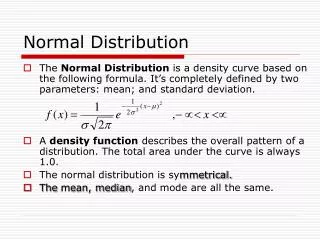
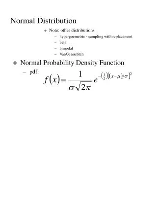
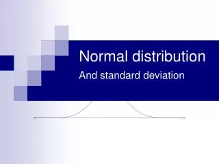
Normal Distribution • Symmetrical, bell-shaped curve • Also known as Gaussian distribution • Point of inflection = 1 standard deviation from mean • Mathematical formula
Since we know the shape of the curve, we can calculate the area under the curve • The percentage of that area can be used to determine the probability that a given value could be pulled from a given distribution • The area under the curve tells us about the probability- in other words we can obtain a p-value for our result (data) by treating it as a normally distributed data set.
Key Areas under the Curve • For normal distributions+ 1 SD ~ 68%+ 2 SD ~ 95%+ 3 SD ~ 99.9%
Problem: • Each normal distribution with its own values of m and s would need its own calculation of the area under various points on the curve
Normal Probability DistributionsStandard Normal Distribution – N(0,1) • We agree to use the standard normal distribution • Bell shaped • =0 • =1 • Note: not all bell shaped distributions are normal distributions
Normal Probability Distribution • Can take on an infinite number of possible values. • The probability of any one of those values occurring is essentially zero. • Curve has area or probability = 1
Normal Distribution • The standard normal distribution will allow us to make claims about the probabilities of values related to our own data • How do we apply the standard normal distribution to our data?
Z-score If we know the population mean and population standard deviation, for any value of X we can compute a z-score by subtracting the population mean and dividing the result by the population standard deviation
Important z-score info • Z-score tells us how far above or below the mean a value is in terms of standard deviations • It is a linear transformation of the original scores • Multiplication (or division) of and/or addition to (or subtraction from) X by a constant • Relationship of the observations to each other remains the same Z = (X-m)/s then X = sZ + m [equation of the general form Y = mX+c]
Probabilities and z scores: z tables • Total area = 1 • Only have a probability from width • For an infinite number of z scores each point has a probability of 0 (for the single point) • Typically negative values are not reported • Symmetrical, therefore area below negative value = Area above its positive value • Always helps to draw a sketch!
Probabilities are depicted by areas under the curve • Total area under the curve is 1 • The area in red is equal to p(z > 1) • The area in blue is equal to p(-1< z <0) • Since the properties of the normal distribution are known, areas can be looked up on tables or calculated on computer.
Strategies for finding probabilities for the standard normal random variable. • Draw a picture of standard normal distribution depicting the area of interest. • Re-express the area in terms of shapes like the one on top of the Standard Normal Table • Look up the areas using the table. • Do the necessary addition and subtraction.
Example • Data come from distribution: m = 10, s = 3 • What proportion fall beyond X=13? • Z = (13-10)/3 = 1 • =normsdist(1) or table 0.1587 • 15.9% fall above 13
Example: IQ • A common example is IQ • IQ scores are theoretically normally distributed. • Mean of 100 • Standard deviation of 15
IQ’s are normally distributed with mean 100 and standard deviation 15. Find the probability that a randomly selected person has an IQ between 100 and 115
Say we have GRE scores are normally distributed with mean 500 and standard deviation 100. Find the probability that a randomly selected GRE score is greater than 620. • We want to know what’s the probability of getting a score 620 or beyond. • p(z > 1.2) • Result: The probability of randomly getting a score of 620 is ~.12
Work time... • What is the area for scores less than z = -1.5? • What is the area between z =1 and 1.5? • What z score cuts off the highest 30% of the distribution? • What two z scores enclose the middle 50% of the distribution? • If 500 scores are normally distributed with mean = 50 and SD = 10, and an investigator throws out the 20 most extreme scores, what are the highest and lowest scores that are retained?
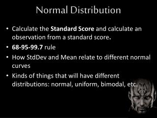
Standard Scores • Z is not the only transformation of scores to be used • First convert whatever score you have to a z score. • New score – new s.d.(z) + new mean • Example- T scores = mean of 50 s.d. 10 • Then T = 10(z) + 50. • Examples of standard scores: IQ, GRE, SAT
Wrap up • Assuming our data is normally distributed allows for us to use the properties of the normal distribution to assess the likelihood of some outcome • This gives us a means by which to determine whether we might think one hypothesis is more plausible than another (even if we don’t get a direct likelihood of either hypothesis)