Normal Distribution
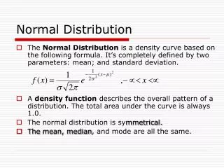
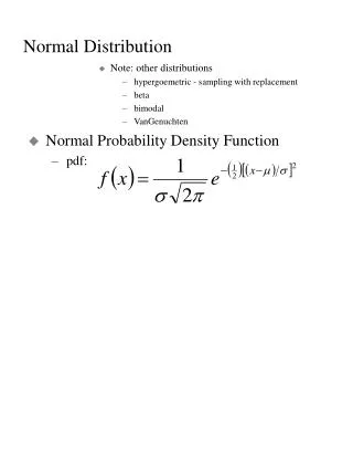
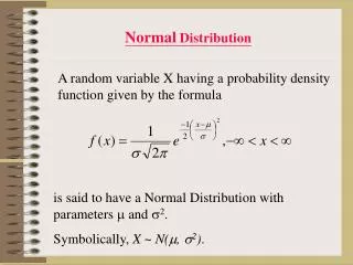
Normal Distribution. A random variable X having a probability density function given by the formula. is said to have a Normal Distribution with parameters and 2 . Symbolically, X ~ N(, 2 ). Properties of Normal Distribution.

Normal Distribution
E N D
Presentation Transcript
Normal Distribution A random variable X having a probability density function given by the formula is said to have a Normal Distribution with parameters and 2. Symbolically, X ~ N(, 2).
Properties of Normal Distribution • The curve extends indefinitely to the left and to the right, approaching the x-axis as x increases in magnitude, i.e. as x , f(x) 0. • The mode occurs atx=. • The curve is symmetric about a vertical axis through the mean • The total area under the curve and above the horizontal axis is equal to 1. i.e.
Empirical Rule (Golden Rule) • The following diagram illustrates relevant areas and associated probabilities of the Normal Distribution. Approximate 68.3% of the area lies within ±, 95.5% of the area lies within ±2, and 99.7% of the area lies within ±3.
For normal curves with the same , they are identical in shapes but the means are centered at different positions along the horizontal axis.
For normal curves with the same mean , the curves are centered at exactly the same position on the horizontal axis, but with different standard deviations , the curves are in different shapes, i.e. the curve with the larger standard deviation is lower and spreads out farther, and the curve with lower standard deviation and the dispersion is smaller.
Normal Table If the random variable X ~ N(, 2), then we can transform all the values of X to the standardized values Z with the mean 0 and variance 1, i.e. Z ~ N(0, 1), on letting
Standardizing Process This can be done by means of the transformation. The mean of Z is zero and the variance is respectively,
Diagrammatic of the Standardizing Process Transforms X ~ N(, 2) to Z ~ N(0, 1). Whenever X is between the values x=x1 and x=x2, Z will fall between the corresponding values z=z1 and z=z2, we have P(x1 < X < x2) = P(z1 < Z < z2). It illustrates by the following diagram:
The normal table can be used to find values like P(Z > a), P(Z < b) and P(a Z b). We illustrate with the following examples. Example 1: P(-1.28 < Z < 0) = ? Solution: P(-1.28 < Z < 0) = P(0 < Z < 1.28) = 0.3997
Example 2: P(Z < -1.28) = ? Solution: P(Z < -1.28) = P(Z > 1.28) = 0.5 – 0.3997 =0.1003
Example 3: P(Z > -1.28) = ? Solution: P(Z > -1.28) = P(Z < 1.28) = 0.5 + 0.3997 = 0.8997
Example 4: P(-2.28 < Z < -1.28) = ? Solution: P(-2.28 < Z < -1.28) = P(1.28 < Z < 2.28) = 0.4887 – 0.3997 = 0.0890
Example 5: P(-1.28 < Z < 2.28) = ? Solution: P(-1.28 < Z < 2.28) = 0.3997 + 0.4887 = 0.8884
Example 6: If P(Z > a) = 0.8, find the value of a? Solution: From the Normal Table A(0.84) 0.3 a - 0.84
Example 7: If P(Z < b) = 0.32, find the value of b? Solution: P(Z < b) = 0.32 P(b < Z < 0) = 0.5 – 0.32 = 0.18 From table, A(0.47) 0.18 b -0.47
Example 8: If P(|Z > c) = 0.1, fin the values of c? Solution: P(|Z > c) = 0.1 P(Z > c) = 0.05 P( c > Z > 0) = 0.5 – 0.05 = 0.45 From table, A(1.645) 0.45 c 1.645
Transformation Example 9: If X ~ N(10, 4), find • P(X 12); • P(9.5 X 11); • P(8.5 X 9) ?
Solution: (b) For the distribution of X with =10, =2 P(9.5 X 11) = P(- 0.25 Z 0.5) = 0.0987 + 0.1915 = 0.2902
Solution: (c) For the distribution of X with =10, =2 P(8.5 X 9) = P(- 0.75 Z - 0.5) = 0.2734 – 0.1915 = 0.0819