Array Methods for Image Formation
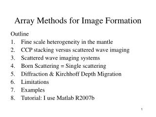
Array Methods for Image Formation. Outline Fine scale heterogeneity in the mantle CCP stacking versus scattered wave imaging Scattered wave imaging systems Born Scattering = Single scattering Diffraction & Kirchhoff Depth Migration Limitations Examples Tutorial: I use Matlab R2007b.

Array Methods for Image Formation
E N D
Presentation Transcript
Array Methods for Image Formation Outline • Fine scale heterogeneity in the mantle • CCP stacking versus scattered wave imaging • Scattered wave imaging systems • Born Scattering = Single scattering • Diffraction & Kirchhoff Depth Migration • Limitations • Examples • Tutorial: I use Matlab R2007b
Summary Data redundancy suppresses noise. Noise is whatever doesn’t fit the scattering model. The image is only as good as the • The velocity model • The completeness of the dataset • The assumptions the imaging system is based on. • We use a single-scattering assumption
SNORCLESubduction forming the Proterozoic continental mantle lithosphere:Lateral advection of massCook et al., (1999)Bostock (1998)
Geometry: Fine scales in the mantle Kellogg and Turcotte, 1994 Allegre and Turcotte, 1986
SUMA: Statistical Upper Mantle Assemblage Reservoirs are distributed Coherent Subduction
Structures from basalt extraction Oman ophiolite
Regional Seismology: PNE DataHighly heterogeneous models of the CL Nielsen et al, 2003, GJI
Two classes of scattered wave imaging systems • Incoherent imaging systems which are frequency and amplitude sensitive. Examples are • Photography • Military Sonar • Some deep crustal reflection seismology • Coherent imaging systems use phase coherence and are therefore sensitive to frequency, amplitude, and phase. Examples are • Medical ultrasound imaging • Military sonar • Exploration seismology • Receiver function imaging • Scattered wave imaging in teleseismic studies • Mixed systems • Sumatra earthquake source by Ishii et al. 2005 See Blackledge, 1989, Quantitative Coherent Imaging: Theory and Applications
Direct imaging with seismic waves Converted Wave Imaging from a continuous, specular, interface Images based on this model of 1 D scattering are referred to as common conversion point stacks or CCP images From Niu and James, 2002, EPSL
CCP Stacking blurs the subsurface The lateral focus is weak
Fresnel Zones and other measures of wave sampling • Fresnel zones • Banana donuts • Wavepaths Are all about the same thing They are means to estimate the sampling volume for waves of finite-frequency, i.e. not a ray, but a wave. Flatté et al., Sound Transmission Through a Fluctuating Ocean
T0=3s 1. Lateral heterogeneity is blurred Moho 2.Mispositioning in depth from average V(z) profile Moho 3. Pulses broaden due to increase in V with z 4. Crustal multiples obscure upper mantle 5. Diffractions stacked out 1p2s 2p1s 1p2s VE=1:1
Scattered wave imaging Based on diffraction theory: Every point in the subsurface causes scattering
/2 Scattered wave imaging improves lateral resolution It also restores dips
USArray: Bigfoot x = 70 km, 7s < T < 30s
Slab Multiples Slab Multiples Mismatch S. Ham, unpublished
Resolution Considerations • Earthquakes are the only inexpensive energy source able to investigate the mantle • Coherent Scattered Wave Imaging provides about an order of magnitude better resolution than travel time tomography. For wavelength • Rscat~/2 versus Rtomo ~ (L)1/2 • For a normalized wavelength and path of 100 • Rscat~ 0.5 versus Rtomo~ 10 • The tomography model provides a smooth background for scattered wave imaging
The receiver function: • Approximately isolates the SV wave from the P wave • Reduces a vector system to a scalar system • Allows use of a scalar imaging equation with P and S calculated separately for single scattering: From Barbara’s lecture:
Three elements of an imaging algorithm • A scattering model • Wave (de)propagator • Diffraction integrals (Wilson et al., 2005) • Kirchhoff Integrals (Bostock, 2002; Levander et al., 2005) • One-way and two-way finite-difference operators (Stanford SEP) • Generalized Radon Transforms (Bostock et al., 2001) • Fourier transforms in space and/or time with phase shifting (Stolt, 1977, Geophysics) • A focusing criteria known as an imaging condition
Depropagator: assume smooth coefficients i.e., c(x,y,z) varies smoothly. Let L be the wave equation Operator for the smooth medium The Green’s function is the inverse operator to the wave equation For a general source:
The Born Approximation Perturbing the velocity field perturbs the wavefield c= c+c -> dL contains dc
Born Scattering Assume a constant density scalar wave equation with a smoothly varying velocity field c(x) Perturb the velocity field
Born Scattering: Solve for the perturbed field to first order The total field consists of two parts, the response to the smooth medium Plus the response to the perturbed medium U The approximate solution satisfies two inhomogenous wave equations. Note that energy is not conserved. It is the scattered field that we use for imaging, noise is anything that doesn’t fit the scattering model
The scattering function for P to S conversion from a heterogeneity Wu and Aki, 1985, Geophysics where Shear wave impedance Fourier Transform relations
Regional Seismology: PNE DataHighly heterogeneous models of the CL Background model is very smooth U senses the smooth field U senses the rough field Nielsen et al, 2003, GJI
Signal Detection: Elastic P to S Scattering from a discrete heterogeneity Wu and Aki, 1985, Geophysics Specular P to S Conversion Aki and Richards, 1980 Levander et al., 2006, Tectonophysics
Definition of an image, from Scales (1995), Seismic Imaging Recall from the RF lecture the definition of a receiver function
A specific depropagator: Diffraction Integrals Start with two scalar wave equations, one homogeneous: and the other the equation for the Green’s function: the response to a singularity in space and time:
Fourier Transform with respect to timegiving two Helmholtz equations wherek =/c
Use the definition of the 3D delta function to sift U(rs,) Given measurements or estimates of two fields U and G, and their normal derivatives on a closed surface S defined by r0, we can predict the value of the field U anywhere within the volume, rs. The integral has been widely used in diffraction theory and forms the basis of a class of seismic migration operators.
We need a Green’s function The constant velocity free space Green’s function is given by The free space asymptotic Green’s function for variable velocity can be written as
Here (r,rs) is the solution to the eikonal equation: And A(r,rs) is the solution to the transport equation: The solution is referred to as a high-frequency or asymptotic solution. Both equations are solved numerically
We want a Green’s function that vanishes on So, or one whose derivative vanishes on So Recenter the coordinate system so that z=0 lies in S A Green’s function which vanishes at z=0 is given by: Where r’s is the image around x of rs. Atz=0 This is also approximately true if So has topography with wavelength long compared to the incident field. This is called Kirchhoff’s approximation.
The diffraction integral becomes Assume that the phase fluctuations are greater than the amplitude fluctuations we can throw away the first term. This is a far field approximation: This is the Rayleigh-Sommerfeld diffraction integral (Sommerfeld, 1932, Optics) If we use it to backward propagate the wavefield, rather than forward propagate it, it is an imaging integral.
Imaging Condition The imaging condition is given by the time it took the source to arrive at the scatterer plus the time it took the scattered waves to arrive at the receiver. If we have an accurate description of c( r) then the waves are focused at the scattering point. (attributed to Jon Claerbout) The image is as good as the velocity model. For an incident P-wave and a scattered S-wave, and an observation at ro, then the image would focus at point r, when
Because the phase is zero at the imaging point, the inverse Fourier transform becomes a frequency sum Recall that U is a receiver function and the desired image is Define
P(x,z) S(x,z)
Sensitivities • Spatial aliasing and Aperture • First Fresnel zone has to be well sampled in a Fourier sense • Generally 2L > ztarget We need lots of receivers Ex: b=3.6, f=0.5, 45 deg Dx = 5 km L~1000 km 400 stations
Data redundancy • Redundancy builds Signal/(Random Noise) as N0.5, where N is the number of data contributing at a given image point: N=Nevent*Nreceiver • Events from different incidence angles, i.e. source distances, suppresses reverberations • Events from different incidence angles reconstruct a larger angular spectrum of the target
Other considerations • A good starting velocity model is required • Use the travel-time tomography model • Data preconditioning • DC removal • Frequency filter • Remove the direct wave and other signals that don’t fit the scattering model • Wavenumber filters (ouch!)
Vp~ 7.75 km/s 1% Partial Melt