Implementation of Stommel Model for Ocean Circulation Using Finite Difference Method
This document presents a prototype finite difference model based on the Stommel problem, focusing on 2D solutions for ocean circulation. It details the wind-driven flow in a rectangular, homogeneous ocean influenced by surface winds, bottom friction, and Coriolis force. The solution showcases the concentration of streamlines at the western boundary due to latitude-based variations in the Coriolis parameter. The implementation is guided by MPI for distributed memory architectures, providing insight into the coding aspects of Fortran 90, including modules, allocatable arrays, and interfaces, for enhanced memory management and optimization.


Implementation of Stommel Model for Ocean Circulation Using Finite Difference Method
E N D
Presentation Transcript
Part 1: Stommel Model – definition and serial implementation • 2D solution to a model problem for Ocean Circulation • Serves as a prototype finite difference model. Illustrates many aspects of a typical code taking advantage of distributed memory computers using MPI.
The Stommel Problem • Wind-driven circulation in a homogeneous rectangular ocean under the influence of surface winds, linearized bottom friction, flat bottom and Coriolis force. • Solution: intense crowding of streamlines towards the western boundary caused by the variation of the Coriolis parameter with latitude
Governing Equations 2 2 ¶ y ¶ y ¶ y ( ) f b g + + = 2 2 x ¶ x y ¶ ¶ y p f s i n ( ) = - a 2L y L L 2 0 0 0 K m = = x y ( 6 ) - 3 1 0 g = * ( 1 1 ) - 2 . 2 5 1 0 b = * ( 9 ) - 1 0 a =
Domain Discretization D e f i n e a g r i d c o n s i s t i n g o f p o i n t s ( x , y ) g i v e n b y i j x i x , i 0 , 1 , . . . . . . . , n x + 1 = D = i y j y , j 0 , 1 , . . . . . . . , n y + 1 = D = j x L ( n x 1 ) D = + x y L ( n y 1 ) D = + y
Domain Discretization (cont’d) Seek to find an approximate solution ( x , y ) a t p o i n t s ( x , y ) : y i i j j ( x , y ) y » y i , j i j
Centered Finite Difference Scheme for the Derivative Operators
Five-point Stencil Approximationfor the Discrete Stommel Model i, j+1 interior grid points: i=1,nx; j=1,ny boundary points: (i,0) & (i,ny+1) ; i=1,nx (0,j) & (nx+1,j) ; j=1,ny i, j i-1, j i+1, j i, j-1
Jacobi Iteration Start with an initial guess for do i = 1, nx; j = 1, ny end do Copy Repeat the process
Implementation Overview /work/Training/examples/stommel/ • Code written in Fortran 90 as well as in C • Uses many features of F90 • Modules instead of commons • Free format • Module with kind precision facility • Interfaces • Allocatable arrays • Array syntax
Free Format • Statements can begin in any column • ! Starts a comment • To continue a line use a “&” on the line to be continued
Modules instead of commons • Modules have a name and can be used in place of named commons • Modules are defined outside of other subroutines • To “include” the variables from a module in a routine you “use” it • The main routine stommel and subroutine jacobi share the variables in module “constants” module constants real dx,dy,a1,a2,a3,a4,a5,a6 end module … program stommel use constants … end program subroutine jacobi use constants … end subroutine jacobi
Kind precision facility Instead of declaring variables real*8 x,y We use real(b8) x,y Where b8 is a constant defined within a module module numz integer,parameter::b8=selected_real_kind(14) end module program stommel use numz real(b8) x,y x=1.0_b8 ...
Why use kind precision facility? Legality Portability Reproducibility Modifiability real*8 x,y is not legal syntax in Fortran 90 Declaring variables “double precision” will give us 16 byte reals on some machines integer,parameter::b8=selected_real_kind(14) real(b8) x,y x=1.0_b8uprecision
Allocatable arrays • We can declare arrays to be allocatable • Allows dynamic memory allocation • Define the size of arrays at run time real(b8),allocatable::psi(:,:) ! our calculation grid real(b8),allocatable::new_psi(:,:) ! temp storage for the grid ! allocate the grid to size nx * ny plus the boundary cells allocate(psi(0:nx+1,0:ny+1)) allocate(new_psi(0:nx+1,0:ny+1))
Interfaces • Similar to C prototypes • Can be part of the routines or put in a module • Provides information to the compiler for optimization • Allows type checking module face interface bc subroutine bc (psi,i1,i2,j1,j2) use numz real(b8),dimension(i1:i2,j1:j2):: psi integer,intent(in):: i1,i2,j1,j2 end subroutine end interface end module program stommel use face ...
Array Syntax Allows assignments of arrays without do loops ! allocate the grid to size nx * ny plus the boundary cells allocate(psi(0:nx+1,0:ny+1)) allocate(new_psi(0:nx+1,0:ny+1)) ! set initial guess for the value of the grid psi=1.0_b8 ! copy from temp to main grid psi(i1:i2,j1:j2)=new_psi(i1:i2,j1:j2)
Program Outline (Fortran) (1) • Module NUMZ - defines the basic real type as 8 bytes • Module INPUT - contains the inputs • nx,ny (Number of cells in the grid) • lx,ly (Physical size of the grid) • alpha,beta,gamma (Input calculation constants) • steps (Number of Jacobi iterations) • Module Constants - contains the invariants of the calculation
Program Outline (2) • Module face - contains the interfaces for the subroutines • bc - boundary conditions • do_jacobi - Jacobi iterations • force - right hand side of the differential equation • Write_grid - writes the grid
Program Outline (3) • Main Program • Get the input • Allocate the grid to size nx * ny plus the boundary cells • Calculate the constants • Set initial guess for the value of the grid • Set boundary conditions • Do the Jacobi iterations • Write out the final grid
C version considerations • To simulate the F90 numerical precision facility we: • #define FLT double • And use FLT as our real data type throughout the rest of the program • We desire flexibility in defining our arrays and matrices • Arbitrary starting indices • Contiguous blocks of memory for 2d arrays • Use routines based on Numerical Recipes in C
Vector allocation routine FLT *vector(INT nl, INT nh) { /* creates a vector with bounds vector[nl:nh]] */ FLT *v; /* allocate the space */ v=(FLT *)malloc((unsigned) (nh-nl+1)*sizeof(FLT)); if (!v) { printf("allocation failure in vector()\n"); exit(1); } /* return a value offset by nl */ return v-nl; }
Matrix allocation routine FLT **matrix(INT nrl,INT nrh,INT ncl,INT nch) /* creates a matrix with bounds matrix[nrl:nrh][ncl:nch] */ /* modified from the book version to return contiguous space */ { INT i; FLT **m; /* allocate an array of pointers */ m=(FLT **) malloc((unsigned) (nrh-nrl+1)*sizeof(FLT*)); if (!m){ printf("allocation failure 1 in matrix()\n"); exit(1);} m -= nrl; /* offset the array of pointers by nrl */ for(i=nrl;i<=nrh;i++) { if(i == nrl){ /* allocate a contiguous block of memroy*/ m[i]=(FLT *) malloc((unsigned) (nrh-nrl+1)*(nch-ncl+1)*sizeof(FLT)); if (!m[i]){ printf("allocation failure 2 in matrix()\n");exit(1); } m[i] -= ncl; /* first pointer points to beginning of the block */ } else { m[i]=m[i-1]+(nch-ncl+1); /* rest of pointers are offset by stride */ } } return m; }
Compiling and running (serial) Compile: xlf90 -O4 stf_00.f -o stf xlc -O4 stc_00.c -o stc Run: poe stf < st.in -nodes 1 -tasks_per_node 1 -rmpool 1 Exercise: measure run times of Fortran and C versions, both optimized (-O4) and unoptimized. Draw conclusions.
Part 2: MPI Version of the Stommel Model code with 1D Decomposition • Choose one of the two dimensions andsubdivide the domain to allow the distribution of the work across a group of distributed memory processors. • We will focus on the principles and techniques usedtodo the MPI work in the model. • Fortran version is used in the presentation.
Introduce the MPI environment • Need to include “mpif.h” to define MPI constants • Need to define our own constants: npes - how many processors are running myid - which processor I am ierr - error code returned by most calls pi_master - the id for the master node Add the following lines: include "mpif.h" integer npes,myid,ierr integer, parameter::mpi_master=0
MPI environment (cont’d) Next need to initialize MPI - add the following to the beginning of your program: call MPI_INIT( ierr ) call MPI_COMM_SIZE(MPI_COMM_WORLD,npes, ierr) call MPI_COMM_RANK(MPI_COMM_WORLD, myid, ierr) write(*,*)’from ‘, myid,’npes=‘,npes At the end of the program add: call MPI_Finalize(ierr) stop
Try it! Compile mpxlf90 –O3 stf_00mod.f -o st_test mpcc –O3 stf_00mod.c -o st_test Run poe st_test < st.in –nodes 1 –tasks_per_node 2 –rmpool 1 Try running again. Do you get the same output? What does running on 2 CPUs really do?
Modify data input We read the data on processor 0 and send to the others if(myid .eq. mpi_master)then read(*,*)nx,ny read(*,*)lx,ly read(*,*)alpha,beta,gamma read(*,*)steps endif We use MPI_BCAST to send the data to the other processors - 8 calls -- one for each variable.
Domain Decomposition (1-D)Physical domain is sliced into sets of columns so that computation in each set of columns will be handled by different processors (In C subdivide in rows) . Why do columns and not rows? Parallel version each processor gets half the cells Serial version all cells on one processor CPU #1 CPU #2
Domain Decomposition (1-D) Fortran 90 allows us to set arbitrary bounds on arrays. Use this feature to break the original grid psi(1:nx,1:ny) into npes subsections of size ny/npes. For 2 CPUs we get the following: CPU#1: psi(1:nx,1:ny/2) CPU#2: psi(1:nx,ny/2+1,ny) • No two processors calculate psi for the same (i,j) • For every processor, psi(i,j) corresponds to psi(i,j) in the serial program. What other ways of doing decomposition can you think of?
Domain Decomposition (1-D) What are ghost cells? To calculate the value for psi(4,4) CPU #1 requires the value from psi(4,3),psi(5,4),psi(3,4),psi(4,5) CPU#1 needs to get (receive) the value of psi(4,5) from CPU#2. CPU#1 will hold the value of psi(4,5) in one of it’s ghost cells. Ghost cells for CPU#1 are created by adding an extra column to the psi array: instead of psi(1:8,1:4) have psi(1:8,1,5) where elements psi(*,5) are ghost cells used to store psi values from CPU#2 CPU #1 CPU #2
Domain Decomposition (1-D) With ghost cells our decomposition becomes... Parallel version each processor gets half the cells plus ghost cells Serial version all cells on one processor CPU #1 CPU #2 ghost cells
Domain Decomposition (1-D) Source code for setting up the distributed grid with ghost cells ! Set the grid indices for each CPU i1=1 i2=nx dj=real(ny)/real(npes) j1=nint(1.0+myid*dj) j2=nint(1.0+(myid+1)*dj)-1 write(*,101)myid,i1,i2,j1,j2 101 format("myid= ",i3,3x,& " (",i3," <= i <= ",i3,") , ", & " (",i3," <= j <= ",i3,")") ! allocate the grid to size i1:i2,j1:j2 but add additional ! cells for boundary values and ghost cells allocate(psi(i1-1:i2+1,j1-1:j2+1)) Since 1-D decomposition only the y-indices change Added to display each CPU’s indices
Ghost cell update Each trip through our main loop we call do_transfer to update the ghost cells. Our main loop becomes... do i=1,steps call do_jacobi(psi,new_psi,mydiff,i1,i2,j1,j2,& for,nx,ny,a1,a2,a3,a4,a5) !update ghost cell values call do_transfer(psi,i1,i2,j1,j2,myid,npes) write(*,*)i,diff enddo
Odd step2 Odd step1 How do we update ghost cells? • Processors send values to and receive from their neighbors. • Need to exchange with left and right neighbors, except processors on far left and right only transfer in 1 direction • Trick 1: to avoid deadlock where all processor try to send, need to split up calls to send and receive: • Even numbered processors: Odd numbered processors: • send to left receive from right • receive from left send to right • receive from right send to left • send to right receive from left Even step1 Odd step1 Even step2 Odd step2 Even step1 Even step2 Trick2: To handle the end CPUs send to MPI_PROC_NULL instead of a real CPU
How do we update ghost cells? ! How many cells are we sending num_x=i2-i1+3 ! Where are we sending them myleft=myid-1 !processor id of CPU on the left myright=myid+1 !processor id of CPU on the right if(myleft .le. -1)myleft=MPI_PROC_NULL if(myright .ge. npes)myright=MPI_PROC_NULL
How do we update ghost cells?For even-numbered processors... if(even(myid))then ! send to left call MPI_SEND(psi(:,j1),num_x,MPI_DOUBLE_PRECISION,& myleft,100,MPI_COMM_WORLD,ierr) ! rec from left call MPI_RECV(psi(:,j1-1),num_x,MPI_DOUBLE_PRECISION,& myleft,100,MPI_COMM_WORLD,status,ierr) ! rec from right call MPI_RECV(psi(:,j2+1),num_x,MPI_DOUBLE_PRECISION,& myright,100,MPI_COMM_WORLD,status,ierr) ! send to right call MPI_SEND(psi(:,j2), num_x,MPI_DOUBLE_PRECISION,& myright,100,MPI_COMM_WORLD,ierr) else
How do we update ghost cells?For odd-numbered processors... Else ! we are on an odd column processor ! rec from right call MPI_RECV(psi(:,j2+1),num_x,MPI_DOUBLE_PRECISION, & myright,100,MPI_COMM_WORLD,status,ierr) ! send to right call MPI_SEND(psi(:,j2), num_x,MPI_DOUBLE_PRECISION, & myright,100,MPI_COMM_WORLD,ierr) ! send to left call MPI_SEND(psi(:,j1), num_x,MPI_DOUBLE_PRECISION, & myleft,100,MPI_COMM_WORLD,ierr) ! rec from left call MPI_RECV(psi(:,j1-1),num_x,MPI_DOUBLE_PRECISION, & myleft,100,MPI_COMM_WORLD,status,ierr) endif
How do we update ghost cells?It’s a 4-stage operation.Example with 4 CPUs:
Other modificationsForce and do_jacobi are not modifiedModify the boundary condition routine so that it only sets values for true boundaries and ignore ghost cells subroutine bc: ! check which CPUs have the edges and assign them the ! correct boundary values if(i1 .eq. 1) psi(i1-1,:)=0.0 !top edge if(i2 .eq. nx) psi(i2+1,:)=0.0 !bottom edge if(j1 .eq. 1) psi(:,j1-1)=0.0 !left edge if(j2 .eq. ny) psi(:,j2+1)=0.0 !right edge Only add if-then statements
Other Modifications : Residual • In our serial program, the routine do_jacobi calculates a residual for each iteration • The residual is the sum of changes to the grid for a jacobi iteration • Now the calculation is spread across all processors • To get the global residual, we can use the MPI_Reduce function call MPI_REDUCE(mydiff,diff,1,MPI_DOUBLE_PRECISION, & MPI_SUM,mpi_master,MPI_COMM_WORLD,ierr) if(myid .eq. mpi_master)write(*,*)i,diff (Since mpi_master now has value of diff, only that CPU writes value)
Our main loop is now…Call the do_jacobi subroutineUpdate the ghost cellsCalculate the global residual do i=1,steps call do_jacobi(psi,new_psi,mydiff,i1,i2,j1,j2) call do_transfer(psi,i1,i2,j1,j2) call MPI_REDUCE(mydiff,diff,1,MPI_DOUBLE_PRECISION, & MPI_SUM,mpi_master,MPI_COMM_WORLD,ierr) if(myid .eq. mpi_master)write(*,*)i,diff enddo
Final change • We change the write_grid subroutine so that each node writes its part of the grid to a different file. • Function unique returns a file name based on a input string and the node number We change the open statement in write_grid to: open(18,file=unique("out1d_"),recl=max(80,15*((jend-jstart)+3)+2))
Unique Unique is the function: function unique(name,myid) implicit none character (len=*) name character (len=20) unique character (len=80) temp integer myid if(myid .gt. 99)then write(temp,"(a,i3)")trim(name),myid else if(myid .gt. 9)then write(temp,"(a,'0',i2)")trim(name),myid else write(temp,"(a,'00',i1)")trim(name),myid endif endif unique=temp return end function unique
Suggested exercises • Study, compile, and run the program stf_01.f and/or stc_01.c on various numbers of processors (2--8). Note timing. • Do decompositionin rows if using Fortran, columns if using C). • Do decomposition so that psi starts at i=1,j=1 for each processor. • Do periodic boundary conditions. • Modify the write_grid routine to output the whole grid from CPU#0
Part 3: 2-D decomposition • The program is almost identical • We now have our grid distributed in a block fashion across the processors instead of striped • We can have ghost cells on 1, 2, 3 or 4 sides of the grid held on a particular processor
2-D Decomposition Example 2-D Decomposition on 50 x 50 grid on 4 processors: CPU #1 CPU #0 Grid on each processor is allocated to: pid= 0 ( 0 <= i <= 26) , ( 0 <= j <= 26) pid= 1 ( 0 <= i <= 26) , ( 25 <= j <= 51) pid= 2 ( 25 <= i <= 51) , ( 0 <= j <= 26) pid= 3 ( 25 <= i <= 51) , ( 25 <= j <= 51) CPU #3 CPU #2 But each processor calculates only for: Where interior grid size is 25,25 pid= 0 ( 1 <= i <= 25) , ( 1 <= j <= 25) pid= 1 ( 1 <= i <= 25) , ( 26 <= j <= 50) pid= 2 (26 <= i <= 50) , ( 1 <= j <= 25) pid= 3 (26 <= i <= 50) , ( 26 <= j <= 50) Extra cells are ghost cells
Only three changes need to be made to our program 1. Given an arbitrary number of processors, find a good topology (number of rows and columns of processors) 2. Make new communicators to allow for easy exchange of ghost cells • Set up communicators so that every processor in the same row is in a given communicator • Set up communicators so that every processor in the same column is in a given communicator 3. Add the up/down communication to do_transfer