Relational Algebra: Query Optimization Techniques
Learn how SQL queries translate to optimized relational algebra plans for efficient execution. Explore key operators and examples in this comprehensive lecture presentation.

Relational Algebra: Query Optimization Techniques
E N D
Presentation Transcript
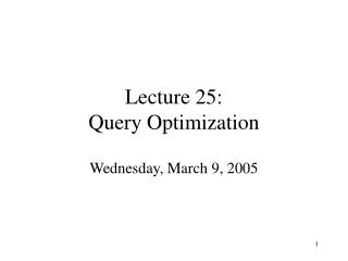
Lecture 7:Query Execution and Optimization Tuesday, February 20, 2007
Outline • Chapters 4, 12-15
DBMS Architecture How does a SQL engine work ? • SQL query relational algebra plan • Relational algebra plan Optimized plan • Execute each operator of the plan
Relational Algebra • Formalism for creating new relations from existing ones • Its place in the big picture: Declartivequerylanguage Algebra Implementation Relational algebraRelational bag algebra SQL,relational calculus
Relational Algebra • Five operators: • Union: • Difference: - • Selection: s • Projection: P • Cartesian Product: • Derived or auxiliary operators: • Intersection, complement • Joins (natural,equi-join, theta join, semi-join) • Renaming: r
1. Union and 2. Difference • R1 R2 • Example: • ActiveEmployees RetiredEmployees • R1 – R2 • Example: • AllEmployees -- RetiredEmployees
What about Intersection ? • It is a derived operator • R1 R2 = R1 – (R1 – R2) • Also expressed as a join (will see later) • Example • UnionizedEmployees RetiredEmployees
3. Selection • Returns all tuples which satisfy a condition • Notation: sc(R) • Examples • sSalary > 40000(Employee) • sname = “Smith”(Employee) • The condition c can be =, <, , >,, <>
4. Projection • Eliminates columns, then removes duplicates • Notation: P A1,…,An(R) • Example: project social-security number and names: • PSSN, Name (Employee) • Output schema: Answer(SSN, Name) Note that there are two parts: Eliminate columns (easy) Remove duplicates (hard) In the “extended” algebra we will separate them.
5. Cartesian Product • Each tuple in R1 with each tuple in R2 • Notation: R1 R2 • Example: • Employee Dependents • Very rare in practice; mainly used to express joins
Relational Algebra • Five operators: • Union: • Difference: - • Selection: s • Projection: P • Cartesian Product: • Derived or auxiliary operators: • Intersection, complement • Joins (natural,equi-join, theta join, semi-join) • Renaming: r
Renaming • Changes the schema, not the instance • Notation: rB1,…,Bn (R) • Example: • rLastName, SocSocNo (Employee) • Output schema: Answer(LastName, SocSocNo)
Renaming Example Employee Name SSN John 999999999 Tony 777777777 • LastName, SocSocNo (Employee) LastName SocSocNo John 999999999 Tony 777777777
Natural Join • Notation: R1 || R2 • Meaning: R1 || R2 = PA(sC(R1 R2)) • Where: • The selection sC checks equality of all common attributes • The projection eliminates the duplicate common attributes
Employee Dependents = PName, SSN, Dname(sSSN=SSN2(Employee x rSSN2, Dname(Dependents)) Natural Join Example Employee Name SSN John 999999999 Tony 777777777 Dependents SSN Dname 999999999 Emily 777777777 Joe Name SSN Dname John 999999999 Emily Tony 777777777 Joe
Natural Join • R= S= • R || S=
Natural Join • Given the schemas R(A, B, C, D), S(A, C, E), what is the schema of R || S ? • Given R(A, B, C), S(D, E), what is R || S ? • Given R(A, B), S(A, B), what is R || S ?
Theta Join • A join that involves a predicate • R1 ||q R2 = sq (R1 R2) • Here q can be any condition
Eq-join • A theta join where q is an equality • R1 ||A=B R2 = s A=B (R1 R2) • Example: • Employee ||SSN=SSN Dependents • Most useful join in practice
Semijoin • R | S = PA1,…,An (R || S) • Where A1, …, An are the attributes in R • Example: • Employee | Dependents
Semijoins in Distributed Databases • Semijoins are used in distributed databases Dependents Employee network Employee ||ssn=ssn (s age>71 (Dependents)) T = PSSNs age>71 (Dependents) R = Employee | T Answer = R || Dependents
seller-ssn=ssn pid=pid buyer-ssn=ssn Complex RA Expressions Pname Person Purchase Person Product Pssn Ppid sname=fred sname=gizmo
Summary on the Relational Algebra • A collection of 5 operators on relations • Codd proved in 1970 that the relational algebra is equivalent to the relational calculus Relational calculus/First order logic/ SQL/declarative language=WHAT Relational algebra/procedural language=HOW =
Operations on Bags A bag = a set with repeated elements All operations need to be defined carefully on bags • {a,b,b,c}{a,b,b,b,e,f,f}={a,a,b,b,b,b,b,c,e,f,f} • {a,b,b,b,c,c} – {b,c,c,c,d} = {a,b,b,d} • sC(R): preserve the number of occurrences • PA(R): no duplicate elimination • = explicit duplicate elimination • Cartesian product, join: no duplicate elimination Important ! Relational Engines work on bags, not sets ! Reading assignment: 5.3 – 5.4
Note: RA has Limitations ! • Cannot compute “transitive closure” • Find all direct and indirect relatives of Fred • Cannot express in RA !!! Need to write C program
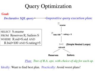
From SQL to RA Purchase(buyer, product, city) Person(name, age) buyer SELECTDISTINCT P.buyer FROM Purchase P, Person Q WHERE P.buyer=Q.name AND P.city=‘Seattle’ AND Q.age > 20 city=‘Seattle’ and age > 20 buyer=name Person Purchase
Also… Purchase(buyer, product, city) Person(name, age) SELECTDISTINCT P.buyer FROM Purchase P, Person Q WHERE P.buyer=Q.name AND P.city=‘Seattle’ AND Q.age > 20 buyer buyer=name city=‘Seattle’ age > 20 Person Purchase
Non-monontone Queries (in class) Purchase(buyer, product, city) Person(name, age) SELECTDISTINCT P.product FROM Purchase P WHERE P.city=‘Seattle’ AND not exists (select * from Purchase P2, Person Q where P2.product = P.product and P2.buyer = Q.name and Q.age > 20)
Extended Logical Algebra Operators(operate on Bags, not Sets) • Union, intersection, difference • Selection s • Projection P • Join |x| • Duplicate elimination d • Grouping g • Sorting t
Logical Query Plan T3(city, c) SELECT city, count(*) FROM sales GROUP BY city HAVING sum(price) > 100 P city, c T2(city,p,c) s p > 100 T1(city,p,c) g city, sum(price)→p, count(*) → c sales(product, city, price) T1, T2, T3 = temporary tables
Logical v.s. Physical Algebra • We have seen the logical algebra so far: • Five basic operators, plus group-by, plus sort • The Physical algebra refines each operator into a concrete algorithm
Physical Plan d Hash-baseddup. elim Purchase(buyer, product, city) Person(name, age) SELECTDISTINCT P.buyer FROM Purchase P, Person Q WHERE P.buyer=Q.name AND P.city=‘Seattle’ AND Q.age > 20 buyer index-join buyer=name sequential scan city=‘Seattle’ age > 20 Purchase Person
Physical Plans Can Be Subtle SELECT * FROM Purchase P WHERE P.city=‘Seattle’ primary-index-join buyer sequential scan city=‘Seattle’ Purchase City-index Where did the join come from ?
Architecture of a Database Engine SQL query Parse Query Logicalplan Select Logical Plan Queryoptimization Select Physical Plan Physicalplan Query Execution
Question in Class Logical operator: Product(pname, cname) || Company(cname, city) Propose three physical operators for the join, assuming the tables are in main memory:
Question in Class Product(pname, cname) |x| Company(cname, city) • 1000000 products • 1000 companies How much time do the following physical operators take if the data is in main memory ? • Nested loop join time = • Sort and merge = merge-join time = • Hash join time =
Cost Parameters The cost of an operation = total number of I/Os result assumed to be delivered in main memory Cost parameters: • B(R) = number of blocks for relation R • T(R) = number of tuples in relation R • V(R, a) = number of distinct values of attribute a • M = size of main memory buffer pool, in blocks NOTE: Book uses M for the number of blocks in R,and B for the number of blocks in main memory
Cost Parameters • Clustered table R: • Blocks consists only of records from this table • B(R) << T(R) • Unclustered table R: • Its records are placed on blocks with other tables • B(R) T(R) • When a is a key, V(R,a) = T(R) • When a is not a key, V(R,a)
Selection and Projection Selection s(R), projection P(R) • Both are tuple-at-a-time algorithms • Cost: B(R) Unary operator Input buffer Output buffer
Hash Tables • Key data structure used in many operators • May also be used for indexes, as alternative to B+trees • Recall basics: • There are n buckets • A hash function f(k) maps a key k to {0, 1, …, n-1} • Store in bucket f(k) a pointer to record with key k • Secondary storage: bucket = block, use overflow blocks when needed
Hash Table Example • Assume 1 bucket (block) stores 2 keys + pointers • h(e)=0 • h(b)=h(f)=1 • h(g)=2 • h(a)=h(c)=3 0 1 2 3 Here: h(x) = x mod 4
Searching in a Hash Table • Search for a: • Compute h(a)=3 • Read bucket 3 • 1 disk access 0 1 2 3
Insertion in Hash Table • Place in right bucket, if space • E.g. h(d)=2 0 1 2 3
Insertion in Hash Table • Create overflow block, if no space • E.g. h(k)=1 • More over-flow blocksmay be needed 0 1 2 3
Hash Table Performance • Excellent, if no overflow blocks • Degrades considerably when number of keys exceeds the number of buckets (I.e. many overflow blocks).
Main Memory Hash Join Hash join: R |x| S • Scan S, build buckets in main memory • Then scan R and join • Cost: B(R) + B(S) • Assumption: B(S) <= M
Main MemoryDuplicate Elimination Duplicate elimination d(R) • Hash table in main memory • Cost: B(R) • Assumption: B(d(R)) <= M


![Query Execution [15]](https://cdn2.slideserve.com/4816696/query-execution-15-dt.jpg)