Efficient Execution of Multi-Query Data Analysis Batches Using Compiler Optimization Strategies
170 likes | 316 Vues
Efficient Execution of Multi-Query Data Analysis Batches Using Compiler Optimization Strategies. Henrique Andrade – http://www.cs.umd.edu/~hcma (in conjunction with Suresh Aryangat, Tahsin Kurc, Joel Saltz, and Alan Sussman) Department of Computer Science University of Maryland

Efficient Execution of Multi-Query Data Analysis Batches Using Compiler Optimization Strategies
E N D
Presentation Transcript
Efficient Execution of Multi-Query Data Analysis Batches Using Compiler Optimization Strategies Henrique Andrade – http://www.cs.umd.edu/~hcma (in conjunction with Suresh Aryangat, Tahsin Kurc, Joel Saltz, and Alan Sussman) Department of Computer ScienceUniversity of Maryland College Park, MD And Department of Biomedical Informatics The Ohio State University Columbus, OH The 16th International Workshop on Languages and Compilers for Parallel Computing College Station, TX – Oct 2-4, 2003
Plenty of scientific data is becoming available • More and more scientific data is being accumulated every day • Sources: Satellites, weather sensors, earthquake sensors, MRI machines, microscopes, etc… • More and more scientific data repositories are becoming available • NASA’s National Space Science Data Center (NSSDC) • NLM’s Visible Human Repository • Brazil’s National Institute for Space Research (INPE) remote sensing data repository • High-level key questions: • How can we locate and visualize the raw data collected by the sensors? • How can we test analytical models for prediction of physical phenomena (e.g., fire prediction in Southern California)? • How can we inspect, analyze, and infer conclusions from a myriad of data from different sensors (e.g., is College Park going to be as rainy as Seattle for too long?) • How can multiple people interact and query these repositories? • How can we leverage the fact that some parts of a dataset are more popular than others (e.g., if one is doing crop yield prediction, Iowa is probably more popular than New Mexico!) to optimize the query execution process? Henrique Andrade (hcma@cs.umd.edu)
Example applications Virtual Microscope ImageProcessing (Pathology) VolumetricReconstruction Surface Groundwater Modeling Kronos Satellite Data Analysis Henrique Andrade (hcma@cs.umd.edu)
Query Batches • The need to handle query batches arises in many situations • Multiple queries may be part of a sense-and-respond system (e.g., calculate the probability of a wildfire in Southern California to active a response from a fire brigade) • Multiple clients may be interacting with the database and queries are batched while the system is busy – Multi-Query Optimization (MQO) • A user may be generating a complex data product like a multimedia visualization that requires coalescing multiple data products • Speeding up the execution of batches of queries • Many scientific datasets have regions of higher interest • Example: agriculture production areas, areas facing risk of wild fires, areas facing deforestation risks, etc. • Regions of higher interest are the target of multiple queries multiple queries on the same parts of a dataset have redundancies less redundancy, faster execution • Key question: how to detect and remove the redundancies from query plans with user-defined aggregation functions and operations Henrique Andrade (hcma@cs.umd.edu)
Set of declarative queries (PostgreSQL) Convert into a set of imperative query descriptions 3-part optimization phase Loop Fusion (LF) Common Sub-expression Elimination (CSE) Dead Code Elimination (DCE) Execution of Optimized Query Plan Our Approach in a Nutshell Henrique Andrade (hcma@cs.umd.edu)
Application: Kronos Kronos • Remote sensing • AVHRR (Advanced Very High Resolution Radiometer) datasets • 5-spectral bands • 1GB per day • Visualization • Multiple correction, compositing algorithms, and cartographic projections • Query attributes • Spatial coordinates • Temporal coordinates • Zoom level • Correction algorithm • Compositing algorithm • Use for: crop yield studies, wild fire prediction, etc. Henrique Andrade (hcma@cs.umd.edu)
A set of PostgreSQL queries is converted into an imperative description PostgreSQL has constructs to support user-defined primitives The imperative query description relies on a canonical loop with the iteration space defined as a multi-dimensional bounding box (the spatio-temporal attributes of a query) The loop body is a collection of assignment statements indicating the execution chain for a particular query The processing unit is a primitive: a user-defined entity with no side effects, registered in the database catalog First Step: Declarative to Imperative Query batch in PostgreSQL Imperative Queries, using canonical loops Henrique Andrade (hcma@cs.umd.edu)
Second step: Loop splitting and fusion Input • Identify the loops with overlapping iteration spaces and merge them • Loop splitting/fusion are the enablers for the other optimizations Two overlapping queries Output Henrique Andrade (hcma@cs.umd.edu)
After fusing the loops, some of the statements in the loop body may become redundant Redundant statement can be replaced by a copy operation Copies are usuallycheaper (I/O and computation) than invoking a primitive Third Step: Common Sub-expression Elimination Input Output Henrique Andrade (hcma@cs.umd.edu)
The elimination of common sub-expressions may generate dead code Statements that are no longer relevant Dead code is dead! Statements can be eliminated, simplifying the query plan The final output can be used by the database virtual machine for execution Fourth Step: Dead Code Elimination Input Output Henrique Andrade (hcma@cs.umd.edu)
Workload Profile 1 Workload Profile 2 Workload Profile 3 Workload Profile 4 New Point-of-Interest 5% 5% 65% 65% Spatial Movement 10% 50% 5% 35% New Resolution 15% 15% 5% 0% Temporal Movement 5% 5% 5% 0% New Correction 25% 5% 5% 0% New Compositing 25% 5% 5% 0% New Compositing Level 15% 15% 10% 0% Experimental Environment Highest probability of data/computation reuse in the batch • Porting Kronos • Rewriting primitives to conform to the database requirements • Dataset • 30GB of AVHRR datasets (January 1992) • Computational environment • 24-processor, 24GB SunFire Solaris machine • Experiments used a single processor (parallel version is under development) • Workload • Synthetic workload (from a Customer Behavior Model Graph) – which defines how queries in a batch are related • 4 different data/computation reuse profiles • 2, 4, 8, 16, 24, and 32-query batches • 256 x 256 pixel window • 2 setups: common sub-expression and loop fusion only (CSE-LF) and common sub-expression, dead code elemination, and loop fusion (CSE-DCE-LF) Transition Lowest probability of data/computation reuse in the batch Henrique Andrade (hcma@cs.umd.edu)
Batch Execution Time Normalized results w.r.t. to no optimizations Relative Batch Execution Time Improvements • Reduction in batch execution time can be as large as 70% with the optimizer: more data/computation reuse in the batch larger reduction • Dead code elimination (DCE) causes a further reduction (irrelevant statements still consume time) cse-lf 100 cse-dce-lf 90 80 70 60 50 Batch Execution Time Reduction (%) 40 30 20 10 0 -10 2 4 8 16 24 32 2 4 8 16 24 32 2 4 8 16 24 32 2 4 8 16 24 32 Workload Profile 1 Workload Profile 2 Workload Profile 3 Workload Profile 4 Workload Profile # / # of queries in the batch Henrique Andrade (hcma@cs.umd.edu)
Average Query Turnaround Time Average Query Turnaround Time off • Although optimizing for batch execution, individual queries are executed faster too! • Decrease can be very significant if reuse potential is high in the batch: query turnaround time can be cut by a factor as large as 2 300 cse-lf 280 260 cse-dce-lf 240 220 200 180 160 Time (s) 140 120 100 80 60 40 20 0 2 4 8 16 24 32 2 4 8 16 24 32 2 4 8 16 24 32 2 4 8 16 24 32 Workload Profile 1 Workload Profile 2 Workload Profile 3 Workload Profile 4 Workload Profile # / # of queries in the batch Henrique Andrade (hcma@cs.umd.edu)
Related Work • The system resulting from this work is built on top of database infrastructure for multi-query optimization for data analysis queries that employs an active semantic data caching scheme (for details [SC 2001, CCGrid 2002, SC 2002, IPDPS 2002, IPDPS 2003]) • Employing compiler optimization strategies for speeding up query execution was thoroughly investigated by Ferreira and Agrawal (multiple publications listed in the paper) • Earlier work on employing algorithmic-level information for multi-query optimization is [Kang, Dietz, Bhargava 1994] Henrique Andrade (hcma@cs.umd.edu)
Conclusions • The optimization process is responsible for a significant decrease in batch and query execution times • From experimental results using a real application • With multiple user-defined primitives • End-to-end optimization: from parsing a declarative query batch up to the virtual machine able to interpret and execute the query plans • Projected extensions • Resource management issues: different (optimized) loop orderings lead to different memory usage patterns • Goal: minimize memory utilization, improve cache locality • Integration with semantic cache: database infrastructure is able to semantically tag and store final and intermediate results of previous queries • Goal: employ the cached aggregates during common sub-expression elimination Henrique Andrade (hcma@cs.umd.edu)
Plan Generation Time off 0.260 cse-lf 0.240 cse-dce-lf 0.220 0.200 0.180 0.160 0.140 Time (s) 0.120 0.100 0.080 0.060 0.040 0.020 0.000 2 4 8 16 24 32 2 4 8 16 24 32 2 4 8 16 24 32 2 4 8 16 24 32 Workload Profile 1 Workload Profile 2 Workload Profile 3 Workload Profile 4 Workload Profile # / # of queries in the batch Time to Generate Batch Plan • Plan generation time is many orders of magnitude smaller than the batch processing time • Interestingly, adding dead code elimination (DCE) causes the plan generation time to drop • Although it requires more processing, it also lowers the number of statements and the complexity of the loops, which cause the optimization process to require less time Henrique Andrade (hcma@cs.umd.edu)
