Query Execution
Query Execution. Where are we?. File organizations: sorted, hashed, heaps. Indexes: hash index, B+-tree Indexes can be clustered or not. Data can be stored in the index or not. Hence, when we access a relation, we can either scan or go through an index: Called an access path.

Query Execution
E N D
Presentation Transcript
Where are we? • File organizations: sorted, hashed, heaps. • Indexes: hash index, B+-tree • Indexes can be clustered or not. • Data can be stored in the index or not. • Hence, when we access a relation, we can either scan or go through an index: • Called an access path.
Current Issues in Indexing • Multi-dimensional indexing: • how do we index regions in space? • Document collections? • Multi-dimensional sales data • How do we support nearest neighbor queries? • Indexing is still a hot and unsolved problem!
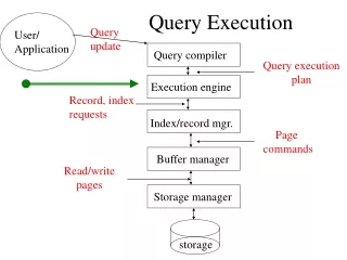
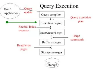
Query Execution Query update User/ Application Query compiler Query execution plan Execution engine Record, index requests Index/record mgr. Page commands Buffer manager Read/write pages Storage manager storage
Query Execution Plans SELECT P.buyer FROM Purchase P, Person Q WHERE P.buyer=Q.name AND Q.city=‘seattle’ AND Q.phone > ‘5430000’ buyer City=‘seattle’ phone>’5430000’ • Query Plan: • logical tree • implementation choice at every node • scheduling of operations. (Simple Nested Loops) Buyer=name Person Purchase (Table scan) (Index scan) Some operators are from relational algebra, and others (e.g., scan, group) are not.
The Leaves of the Plan: Scans • Table scan: iterate through the records of the relation. • Index scan: go to the index, from there get the records in the file (when would this be better?) • Sorted scan: produce the relation in order. Implementation depends on relation size.
How do we combine Operations? • The iterator model. Each operation is implemented by 3 functions: • Open: sets up the data structures and performs initializations • GetNext: returns the the next tuple of the result. • Close: ends the operations. Cleans up the data structures. • Enables pipelining! • Contrast with data-driven materialize model. • Sometimes it’s the same (e.g., sorted scan).
Implementing Relational Operations • We will consider how to implement: • Selection ( ) Selects a subset of rows from relation. • Projection ( ) Deletes unwanted columns from relation. • Join ( ) Allows us to combine two relations. • Set-difference Tuples in reln. 1, but not in reln. 2. • UnionTuples in reln. 1 and in reln. 2. • Aggregation (SUM, MIN, etc.) and GROUP BY
Schema for Examples Purchase (buyer:string, seller: string, product: integer), Person (name:string, city:string, phone: integer) • Purchase: • Each tuple is 40 bytes long, 100 tuples per page, 1000 pages (i.e., 100,000 tuples, 4MB for the entire relation). • Person: • Each tuple is 50 bytes long, 80 tuples per page, 500 pages (i.e, 40,000 tuples, 2MB for the entire relation).
SELECT * FROM Person R WHERE R.phone < ‘543%’ Simple Selections • Of the form • With no index, unsorted: Must essentially scan the whole relation; cost is M (#pages in R). • With an index on selection attribute: Use index to find qualifying data entries, then retrieve corresponding data records. (Hash index useful only for equality selections.) • Result size estimation: (Size of R) * reduction factor. More on this later.
Using an Index for Selections • Cost depends on #qualifying tuples, and clustering. • Cost of finding qualifying data entries (typically small) plus cost of retrieving records. • In example, assuming uniform distribution of phones, about 54% of tuples qualify (500 pages, 50000 tuples). With a clustered index, cost is little more than 500 I/Os; if unclustered, up to 50000 I/Os! • Important refinement for unclustered indexes: 1. Find and sort the rid’s of the qualifying data entries. 2. Fetch rids in order. This ensures that each data page is looked at just once (though # of such pages likely to be higher than with clustering).
Two Approaches to General Selections • First approach:Find the most selective access path, retrieve tuples using it, and apply any remaining terms that don’t match the index: • Most selective access path: An index or file scan that we estimate will require the fewest page I/Os. • Consider city=“seattle AND phone<“543%” : • A hash index on city can be used; then, phone<“543%” must be checked for each retrieved tuple. • Similarly, a b-tree index on phone could be used; city=“seattle” must then be checked.
Intersection of Rids • Second approach • Get sets of rids of data records using each matching index. • Then intersect these sets of rids. • Retrieve the records and apply any remaining terms.
Implementing Projection SELECTDISTINCT R.name, R.phone FROM Person R • Two parts: (1) remove unwanted attributes, (2) remove duplicates from the result. • Refinements to duplicate removal: • If an index on a relation contains all wanted attributes, then we can do an index-only scan. • If the index contains a subset of the wanted attributes, you can remove duplicates locally.
Equality Joins With One Join Column SELECT * FROM Person R, Purchase S WHERE R.name=S.buyer • R S is a common operation. The cross product is too large. Hence, performing R S and then a selection is too inefficient. • Assume: M pages in R, pR tuples per page, N pages in S, pS tuples per page. • In our examples, R is Person and S is Purchase. • Cost metric: # of I/Os. We will ignore output costs.
Discussion • How would you implement join?
Simple Nested Loops Join For each tuple r in R do for each tuple s in S do if ri == sj then add <r, s> to result • For each tuple in the outer relation R, we scan the entireinner relation S. • Cost: M + (pR * M) * N = 1000 + 100*1000*500 I/Os: 140 hours! • Page-oriented Nested Loops join: For each page of R, get each page of S, and write out matching pairs of tuples <r, s>, where r is in R-page and S is in S-page. • Cost: M + M*N = 1000 + 1000*500 (1.4 hours)
Index Nested Loops Join foreach tuple r in R do foreach tuple s in S where ri == sj do add <r, s> to result • If there is an index on the join column of one relation (say S), can make it the inner. • Cost: M + ( (M*pR) * cost of finding matching S tuples) • For each R tuple, cost of probing S index is about 1.2 for hash index, 2-4 for B+ tree. Cost of then finding S tuples depends on clustering. • Clustered index: 1 I/O (typical), unclustered: up to 1 I/O per matching S tuple.
Examples of Index Nested Loops • Hash-index on name of Person (as inner): • Scan Purchase: 1000 page I/Os, 100*1000 tuples. • For each Person tuple: 1.2 I/Os to get data entry in index, plus 1 I/O to get (the exactly one) matching Person tuple. Total: 220,000 I/Os. (36 minutes) • Hash-index on buyer of Purchase (as inner): • Scan Person: 500 page I/Os, 80*500 tuples. • For each Person tuple: 1.2 I/Os to find index page with data entries, plus cost of retrieving matching Purchase tuples. Assuming uniform distribution, 2.5 purchases per buyer (100,000 / 40,000). Cost of retrieving them is 1 or 2.5 I/Os depending on clustering.
. . . Block Nested Loops Join • Use one page as an input buffer for scanning the inner S, one page as the output buffer, and use all remaining pages to hold ``block’’ of outer R. • For each matching tuple r in R-block, s in S-page, add <r, s> to result. Then read next R-block, scan S, etc. Join Result R & S Hash table for block of R (k < B-1 pages) . . . . . . Output buffer Input buffer for S
Sort-Merge Join (R S) i=j • Sort R and S on the join column, then scan them to do a ``merge’’ on the join column. • Advance scan of R until current R-tuple >= current S tuple, then advance scan of S until current S-tuple >= current R tuple; do this until current R tuple = current S tuple. • At this point, all R tuples with same value and all S tuples with same value match; output <r, s> for all pairs of such tuples. • Then resume scanning R and S.
Cost of Sort-Merge Join • R is scanned once; each S group is scanned once per matching R tuple. • Cost: M log M + N log N + (M+N) • The cost of scanning, M+N, could be M*N (unlikely!) • With 35, 100 or 300 buffer pages, both Person and Purchase can be sorted in 2 passes; total: 7500. (75 seconds).
Original Relation Partitions OUTPUT 1 1 2 INPUT 2 hash function h . . . B-1 B-1 B main memory buffers Disk Disk Partitions of R & S Join Result Hash table for partition Ri (k < B-1 pages) hash fn h2 h2 Output buffer Input buffer for Si B main memory buffers Disk Disk Hash-Join • Partition both relations using hash fn h: R tuples in partition i will only match S tuples in partition i. • (if partition is bigger than B-2, do it again) • Read in a partition of R, hash it using h2 (<> h!). Scan matching partition of S, search for matches.
Cost of Hash-Join • In partitioning phase, read+write both relations; 2(M+N). In matching phase, read both relations; M+N I/Os. • In our running example, this is a total of 4500 I/Os. (45 seconds!) • Sort-Merge Join vs. Hash Join: • Given a minimum amount of memory both have a cost of 3(M+N) I/Os. Hash Join superior on this count if relation sizes differ greatly. Also, Hash Join shown to be highly parallelizable. • Sort-Merge less sensitive to data skew; result is sorted.
Double Pipelined Join (Tukwila) Hash Join • Partially pipelined: no output until inner read • Asymmetric (inner vs. outer) — optimization requires source behavior knowledge • Double Pipelined Hash Join • Outputs data immediately • Symmetric — requires less source knowledge to optimize


![Query Execution [15]](https://cdn2.slideserve.com/4816696/query-execution-15-dt.jpg)