Database Query Execution
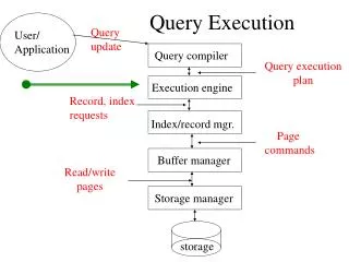
Database Query Execution. Zack Ives CSE 544 - Principles of DBMS Ullman Chapter 6, Query Execution Spring 1999. Query Execution. Inputs: Query execution plan from optimizer Data from source relations Indices Outputs: Query results Data distribution statistics (Also use temp storage).


Database Query Execution
E N D
Presentation Transcript
Database Query Execution Zack Ives CSE 544 - Principles of DBMS Ullman Chapter 6, Query Execution Spring 1999
Query Execution • Inputs: • Query execution plan from optimizer • Data from source relations • Indices • Outputs: • Query results • Data distribution statistics • (Also use temp storage)
Query Plans • Data-flow tree (or graph) of relational algebra operators • Statically pre-compiled vs. dynamic decisions: • “Choose nodes” • Competition • Fragments JoinSymbol = Northwest.CoSymbol JoinPressRel.Symbol = Clients.Symbol ProjectCoSymbol SelectClient = “Atkins” ScanNorthwest Scan PressRel Scan Clients
Plan Execution • Execution granularity & parallelism: • Pipelining vs. blocking • Threads • Materialization • Execution flow: • Iterator/top-down • Data-driven/bottom-up JoinSymbol = Northwest.CoSymbol JoinPressRel.Symbol = Clients.Symbol ProjectCoSymbol SelectClient = “Atkins” ScanNorthwest Scan PressRel Scan Clients
Data-Driven Execution • Schedule leaves (generally parallel or distributed system) • Leaves feed data “up” tree; may need to buffer • Good for slow sources or parallel/distributed • Often less efficient than iterator w.r.t. memory and CPU JoinSymbol = Northwest.CoSymbol JoinPressRel.Symbol = Clients.Symbol ProjectCoSymbol SelectClient = “Atkins” Scan PressRel Scan Clients ScanNorthwest
The Iterator Model • Execution begins at root • open, getNext, close • Propagate calls to children Non-pipelined operation may require multiple getNexts • Efficient scheduling & resource usage • Poor if slow sources (getNext may block) JoinSymbol = Northwest.CoSymbol JoinPressRel.Symbol = Clients.Symbol ProjectCoSymbol SelectClient = “Atkins” Scan PressRel Scan Clients ScanNorthwest
Tukwila Modified Iterator Model • Same operations open, getNext, close • Some operators multithreaded • Use buffering and synchronization • Schedule work while blocked • Multithreaded operators need more memory JoinSymbol = Northwest.CoSymbol JoinPressRel.Symbol = Clients.Symbol ProjectCoSymbol SelectClient = “Atkins” Scan PressRel Scan Clients ScanNorthwest
The Cost of Execution • Costs very important to the optimizer • It must search for low-cost query execution plan • Statistics: • Cardinalities • Histograms (estimate selectivities) • Impact of data integration? • I/O vs. computation costs • Time-to-first-tuple vs. completion time
Reducing Costs with Buffering • Read a page/block at a time • Should look familiar to OS people! • Use a page replacement strategy: • LRU (not as good as you might think) • MRU (good for one-time sequential scans) • Clock • etc. • Note that we have more knowledge than OS to predict paging behavior • e.g. one-time scan should use MRU • Can also prefetch when appropriate Tuple Reads/Writes Buffer Mgr
Select Operator • If unsorted & no index, check against predicate: Read tuple While tuple doesn’t meet predicate Read tuple Return tuple • Sorted data: can stop after particular value encountered • Indexed data: apply predicate to index, if possible • If predicate is: • conjunction: may use indexes and/or scanning loop above (may need to sort/hash to compute intersection) • disjunction: may use union of index results, or scanning loop
Project Operator • Simple scanning method often used if no index: Read tuple While more tuples Output specified attributes Read tuple • Duplicate removal may be necessary • Partition output into separate files by bucket, do duplicate removal on those • May need to use recursion • If have many duplicates, sorting may be better • Can sometimes do index-only scan, if projected attributes are all indexed
The Simplest Join — Nested-Loops • Requires two nested loops: For each tuple in outer relationFor each tuple in inner, compareIf match on join attribute, output • Block nested loops join: read & match page at a time • What if join attributes are indexed? Index nested-loops join • Very simple to implement • Inefficient if size of inner relation > memory (keep swapping pages); requires sequential search for match Join outer inner
Sort-Merge Join • First sort data based on join attributes • Use an external sort (as previously described), unless data is already ordered Merge and join the files, reading sequentially a block at a time • Maintain two file pointers; advance pointer that’s pointing at guaranteed non-matches • Allows joins based on inequalities (non-equijoins) • Very efficient for presorted data • Not pipelined unless data is presorted
Hashing it Out: Hash-Based Joins • Allows (at least some) pipelining of operations with equality comparisons (e.g. equijoin, union) • Sort-based operations block, but allow range and inequality comparisons • Hash joins usually done with static number of hash buckets • Alternatives use directories, are more complex: • Extendible hashing • Linear hashing • Generally have fairly long overflow chains
Hash Join Read entire inner relation into hash table (join attributes as key) For each tuple from outer, look up in hash table & join • Very efficient, very good for databases • Not fully pipelined • Supports equijoins only • Data integration?
Overflowing Memory - GRACE • Two possible strategies: • Overflow prevention (prevent from happening) • Overflow resolution (handle overflow when it occurs) • GRACE hash Write each bucket to separate file Finish reading inner, swapping tuples to appropriate files Read outer, swapping tuples to overflow files matching those from inner Recursively GRACE hash join matching outer & inner overflow files
Overflowing Memory - Hybrid Hash • A “lazy” version of the GRACE hash: When memory overflows, only swap a subset of the tables Continue reading inner relation and building table (sending tuples to buckets on disk as necessary) Read outer, joining with buckets in memory or swapping to disk as appropriate Join the corresponding overflow files, using recursion
Double-Pipelined Join • Two hash tables • As a tuple comes in, add to the appropriate side & join with opposite table • Fully pipelined, data-driven • Needs more memory
Overflow Resolution in the DPJoin • Requires a bunch of ugly bookkeeping! Need to mark tuples depending on state of opposite bucket - this lets us know whether they need to be joined later • Tukwila “Incremental left flush” strategy • Pause reading from outer relation, swap some of its buckets • Finish reading from inner; still join with left-side hash table if possible, or swap to disk • Read outer relation, join with inner’s hash table • Read from overflow files and join as in hybrid hash join
Overflow Resolution, Pt. II • Tukwila “Symmetric flush” strategy: • Flush all tuples for the same bucket from both sides • Continue joining; when done, join overflow files by hybrid hash • Urhan and Franklin’s X-Join • Flush buckets from either relation • If stalled, start trying to join from overflow files • Needs lots of really nasty bookkeeping
The Semi-Join/Dependent Join • Take attributes from left and feed to the right source as input/filter • Important in data integration • Simple method: for each tuple from left send to right source get data back, join • More complex: • Hash “cache” of attributes & mappings • Don’t send attribute already seen JoinA.x = B.y A x B
Issues in Choosing Joins • Goal: minimize I/O costs! • Is the data pre-sorted? • How much memory do I have and need? Selectivity estimates • Inner relation vs. outer relation • Am I doing an equijoin or some other join? • Is pipelining important? • How confident am I in my estimates? • Partition such that partition files don’t overflow!
Sets vs. Bags • Operations requiring set semantics • Duplicate removal • Union • Difference • Methods • Indices • Sorting • Hybrid hashing


![Query Execution [15]](https://cdn2.slideserve.com/4816696/query-execution-15-dt.jpg)