Download
1 / 33
330 likes | 357 Vues
Lecture 24 Query Execution. Monday, November 28, 2005. Outline. Partitioned-base Hash Algorithms External Sorting Sort-based Algorithms. Relation R. Partitions. OUTPUT. 1. 1. 2. INPUT. 2. hash function h. M-1. M-1. M main memory buffers. Disk. Disk.

E N D
Lecture 24Query Execution Monday, November 28, 2005
Outline • Partitioned-base Hash Algorithms • External Sorting • Sort-based Algorithms
Relation R Partitions OUTPUT 1 1 2 INPUT 2 hash function h . . . M-1 M-1 M main memory buffers Disk Disk Two Pass Algorithms Based on Hashing • Idea: partition a relation R into buckets, on disk • Each bucket has size approx. B(R)/M 1 2 B(R) • Does each bucket fit in main memory ? • Yes if B(R)/M <= M, i.e. B(R) <= M2
Hash Based Algorithms for d • Recall: d(R) = duplicate elimination • Step 1. Partition R into buckets • Step 2. Apply d to each bucket (may read in main memory) • Cost: 3B(R) • Assumption:B(R) <= M2
Hash Based Algorithms for g • Recall: g(R) = grouping and aggregation • Step 1. Partition R into buckets • Step 2. Apply g to each bucket (may read in main memory) • Cost: 3B(R) • Assumption:B(R) <= M2
Partitioned Hash Join R |x| S • Step 1: • Hash S into M buckets • send all buckets to disk • Step 2 • Hash R into M buckets • Send all buckets to disk • Step 3 • Join every pair of buckets
Original Relation Partitions OUTPUT 1 1 2 INPUT 2 hash function h . . . M-1 M-1 B main memory buffers Disk Disk Partitions of R & S Join Result Hash table for partition Si ( < M-1 pages) hash fn h2 h2 Output buffer Input buffer for Ri B main memory buffers Disk Disk Hash-Join • Partition both relations using hash fn h: R tuples in partition i will only match S tuples in partition i. • Read in a partition of R, hash it using h2 (<> h!). Scan matching partition of S, search for matches.
Partitioned Hash Join • Cost: 3B(R) + 3B(S) • Assumption: min(B(R), B(S)) <= M2
Hybrid Hash Join Algorithm • Partition S into k buckets t buckets S1 , …, St stay in memory k-t buckets St+1, …, Sk to disk • Partition R into k buckets • First t buckets join immediately with S • Rest k-t buckets go to disk • Finally, join k-t pairs of buckets: (Rt+1,St+1), (Rt+2,St+2), …, (Rk,Sk)
Hybrid Join Algorithm • How to choose k and t ? • Choose k large but s.t. k <= M • Choose t/k large but s.t. t/k * B(S) <= M • Moreover: t/k * B(S) + k-t <= M • Assuming t/k * B(S) >> k-t: t/k = M/B(S)
Hybrid Join Algorithm • How many I/Os ? • Cost of partitioned hash join: 3B(R) + 3B(S) • Hybrid join saves 2 I/Os for a t/k fraction of buckets • Hybrid join saves 2t/k(B(R) + B(S)) I/Os • Cost: (3-2t/k)(B(R) + B(S)) = (3-2M/B(S))(B(R) + B(S))
Hybrid Join Algorithm • Question in class: what is the real advantage of the hybrid algorithm ?
The I/O Model of Computation • In main memory: CPU time • Big O notation ! • In databases time is dominated by I/O cost • Big O too, but for I/O’s • Often big O becomes a constant • Consequence: need to redesign certain algorithms • See sorting next
Sorting • Problem: sort 1 GB of data with 1MB of RAM. • Where we need this: • Data requested in sorted order (ORDER BY) • Needed for grouping operations • First step in sort-merge join algorithm • Duplicate removal • Bulk loading of B+-tree indexes.
2-Way Merge-sort:Requires 3 Buffers in RAM • Pass 1: Read a page, sort it, write it. • Pass 2, 3, …, etc.: merge two runs, write them Runs of length 2L Runs of length L INPUT 1 OUTPUT INPUT 2 Main memory buffers Disk Disk
Two-Way External Merge Sort • Assume block size is B = 4Kb • Step 1 runs of length L = 4Kb • Step 2 runs of length L = 8Kb • Step 3 runs of length L = 16Kb • . . . . . . • Step 9 runs of length L = 1MB • . . . • Step 19 runs of length L = 1GB (why ?) Need 19 iterations over the disk data to sort 1GB
Can We Do Better ? • Hint:We have 1MB of main memory, but only used 12KB
Cost Model for Our Analysis • B(R): size of R in number of blocks • M: Size of main memory (in # of blocks) • E.g. block size = 4KB then: • B(R) = 250000 • M = 250
External Merge-Sort • Phase one: load M bytes in memory, sort • Result: runs of length M bytes ( 1MB ) M . . . . . . Disk Disk M bytes of main memory
Phase Two • Merge M – 1 runs into a new run (250 runs ) • Result: runs of length M (M – 1) bytes (250^2) Input 1 . . . . . . Input 2 Output . . . . Input M/B Disk Disk M bytes of main memory
Phase Three • Merge M – 1 runs into a new run • Result: runs of length M (M – 1)2 Input 1 . . . . . . Input 2 Output . . . . Input M/B Disk Disk M bytes of main memory
Cost of External Merge Sort • Number of passes: • How much data can we sort with 10MB RAM? • 1 pass 10MB data • 2 passes 25GB data • Can sort everything in 2 or 3 passes !
External Merge Sort • The xsort tool in the XML toolkit sorts using this algorithm • Can sort 1GB of XML data in about 8 minutes
Two-Pass Algorithms Based on Sorting • Assumption: multi-way merge sort needs only two passes • Assumption: B(R)<= M2 • Cost for sorting: 3B(R)
Two-Pass Algorithms Based on Sorting Duplicate elimination d(R) • Trivial idea: sort first, then eliminate duplicates • Step 1: sort chunks of size M, write • cost 2B(R) • Step 2: merge M-1 runs, but include each tuple only once • cost B(R) • Total cost: 3B(R), Assumption: B(R)<= M2
Two-Pass Algorithms Based on Sorting Grouping: ga, sum(b) (R) • Same as before: sort, then compute the sum(b) for each group of a’s • Total cost: 3B(R) • Assumption: B(R)<= M2
Two-Pass Algorithms Based on Sorting x = first(R) y = first(S) While (_______________) do{ case x < y: output(x) x = next(R) case x=y: case x > y;} R ∪ S Completethe programin class:
Two-Pass Algorithms Based on Sorting x = first(R) y = first(S) While (_______________) do{ case x < y: case x=y: case x > y;} R ∩ S Completethe programin class:
Two-Pass Algorithms Based on Sorting x = first(R) y = first(S) While (_______________) do{ case x < y: case x=y: case x > y;} R - S Completethe programin class:
Two-Pass Algorithms Based on Sorting Binary operations: R ∪ S, R ∩ S, R – S • Idea: sort R, sort S, then do the right thing • A closer look: • Step 1: split R into runs of size M, then split S into runs of size M. Cost: 2B(R) + 2B(S) • Step 2: merge M/2 runs from R; merge M/2 runs from S; ouput a tuple on a case by cases basis • Total cost: 3B(R)+3B(S) • Assumption: B(R)+B(S)<= M2
Two-Pass Algorithms Based on Sorting R(A,C) sorted on AS(B,D) sorted on B x = first(R) y = first(S) While (_______________) do{ case x.A < y.B: case x.A=y.B: case x.A > y.B;} R |x|R.A =S.B S Completethe programin class:
Two-Pass Algorithms Based on Sorting Join R |x| S • Start by sorting both R and S on the join attribute: • Cost: 4B(R)+4B(S) (because need to write to disk) • Read both relations in sorted order, match tuples • Cost: B(R)+B(S) • Difficulty: many tuples in R may match many in S • If at least one set of tuples fits in M, we are OK • Otherwise need nested loop, higher cost • Total cost: 5B(R)+5B(S) • Assumption: B(R)<= M2, B(S)<= M2
Two-Pass Algorithms Based on Sorting Join R |x| S • If the number of tuples in R matching those in S is small (or vice versa) we can compute the join during the merge phase • Total cost: 3B(R)+3B(S) • Assumption: B(R)+ B(S)<= M2