Query Execution

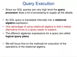
1. Query Execution • Since our SQL queries are very high level the query processor does a lot of processing to supply all the details. • An SQL query is translated internally into a relational algebra expression. • One advantage of using relational algebra is that it makes alternative forms of a query easier to explore. • The different algebraic expressions for a query are called logical query plans. • We will focus first on the methods for execution of the operations of the relational algebra.

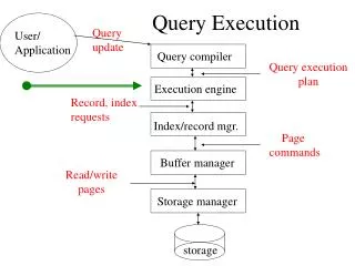
2. Query Compilation (Chapter 16) Query execution (Chapter 15)

3. Preview of Query Compilation • Parsing: read SQL, output relational algebra tree • Query rewrite: Transform tree to a form, which is more efficient to evaluate • Physical plan generation: select implementation for each operator in tree, and for passing results up the tree. • In this chapter we will focus on the implementation for each operator.

4. Relational algebra for real SQL • Basic SELECT-FROM-WHERE queries correspond to (( ..  ..  ..)) in relational algebra • For full SQL support we need additional constructs • A relation in algebra is a set • A relation in SQL might be a bag • Bag = set with duplicates allowed

5. Relational Algebra (RA) on bags • RA union, intersection and difference correspond to UNION, INTERSECT, and EXCEPT in SQL • These are in fact set operators in SQL. If you want bag versions use ALL. • The selection corresponds to the WHERE-clause in SQL • The projection corresponds to SELECT-clause • The product corresponds to FROM-clause • The join’s corresponds to JOIN, NATURAL JOIN, and OUTER JOIN in the SQL2 standard • The duplicate elimination corresponds to DISTINCT in SELECT-clause • The grouping corresponds to GROUP BY • The sorting corresponds to ORDER BY

6. Bag union, intersection, and difference • Card(t,R) means the number of occurrences of tuple t in relation R • Card(t, RS) = Card(t,R) + Card(t,S) • Card(t,RS) = min{Card(t,R), Card(t,S)} • Card(t,R–S) = max{Card(t,R)–Card(t,S), 0} • Example: R= {A,B,B}, S = {C,A,B,C} • R  S = {A,A,B,B,B,C,C} • R  S = {A,B} • R – S = {B}

7. Beware: Bag Laws != Set Laws • Not all algebraic laws that hold for sets also hold for bags. • For one example, the commutative law for union (R S = SR ) does hold for bags. • Since addition is commutative, adding the number of times that tuple x appears in R and S doesn’t depend on the order of R and S. • Set union is idempotent, meaning that SS = S. • However, for bags, if x appears n times in S, then it appears 2n times in SS. • Thus SS != S in general.

8. Selection -- • The condition C might involve • Arithmetic (+,-, ) or string operators such as LIKE • Comparison between terms, e.g. a < b or a+b = 10. • Boolean connectives AND, OR, and NOT • Example: R = a b ---- 2 3 4 5 2 3 a b ---- 0 1 2 3 4 5 2 3 a b ---- 4 5

9. Projection -- Argument L of  is a sequence of elements of the following form: • A single attribute in R, or • An expression x  y, where x and y are attribute names, or • An expression E  z, where E is an expression involving attributes in R and z is a new attribute name not in R • Example: R = a b c ------ 0 1 2 0 1 2 3 4 5 a x ---- 0 3 0 3 3 9 x y ---- 1 1 1 1 1 1

10. R  S = A R.BS.B C 1 2 3 4 1 2 7 8 5 6 3 4 5 6 7 8 1 2 3 4 1 2 7 8 Product --  R( A, B ) S( B, C ) 1 2 3 4 5 6 7 8 1 2 • Each copy of the tuple (1,2) of R is being paired each tuple of S. • So, the duplicates do not an effect on the way we compute the product.

11. Natural Join • The natural join of R and S can be expressed by • starting with the product R  S, • then apply the selection operator with a condition C of the form • R.A1=S.A1AND R.A2=S.A2AND…AND R.An=S.An • where A1,A2,…,An are all the attributes appearing in the schema of both R and S. Finally, we must project out one copy of each of the equated attributes. • R C S = L(C( R  S)) • Where L is the list of attributes in Rfollowed by the list of attributes in S that are not in R.

12. Theta-Join R R.B<S.B S = A R.B S.B C 1 2 3 4 1 2 7 8 5 6 7 8 1 2 3 4 1 2 7 8 R( A, B ) S( B, C ) 1 2 3 4 5 6 7 8 1 2 • Again, each copy of the tuple (1,2) of R is being paired each tuple of S and they join succesfully. • So, the duplicates do not an effect on the way we compute the theta join.

13. (R) = A B 1 2 3 4 Duplicate Elimination • R1 := (R2). • R1 consists of one copy of each tuple that appears in R2 one or more times. R = A B 1 2 3 4 1 2

14. Grouping Operator • R1 := L (R2). L is a list of elements that are either: • Individual (grouping ) attributes. • AGG(A), where AGG is one of the aggregation operators and A is an attribute. • The most important examples: SUM, AVG, COUNT, MIN, and MAX. SELECT starName, MIN(year) AS minYear FROM StarsIn GROUP BY starName HAVING COUNT(title) >= 3;

15. Applying L(R) • Group R according to all the grouping attributes on list L. • That is, form one group for each distinct list of values for those attributes in R. • Within each group, compute AGG(A) for each aggregation on list L. • Result has grouping attributes and aggregations as attributes. • There is one tuple for each list of values for the grouping attributes and their group’s aggregations.

16. Then, average C within groups: A B AVG(C) 1 2 4 4 5 6 First, group R : A B C 1 2 3 1 2 5 4 5 6 Example: Grouping/Aggregation R = A B C 1 2 3 4 5 6 1 2 5 A,B,AVG(C) (R) = ??

17. Example: Grouping/Aggregation • StarsIn(title, year, starName) • Suppose we want, for each star who has appeared in at least three movies the earliest year in which he appeared. • First we group, using starName as a grouping attribute. • Then, we have to compute the MIN(year) for each group. • However, we need also compute COUNT(title) aggregate for each group, in order to filter out those stars with less than three movies. • ctTitle>3[starName,MIN(year)minYear,COUNT(title)ctTitle(StarsIn)

18. Expression trees MovieStar(name, addr, gender, birthdate) StarsIn(title, year, starName) SELECT title, birthdate FROM MovieStar, StarsIn WHERE year = 1996 AND Gender = ‘F’ AND starName = name;

19. How to generate such alternative expression trees will be Chapter 16. • Join method? • Can we pipeline the result of one or both selections, and avoid storing the result on disk temporarily? • Are there indexes on MovieStar.gender and/or StarsIn.year that will make the 's efficient?

20. Physical query plan operators • Physical query plans are built from physical operators. • Often the physical operators are particular implementations of the relational algebra operators. • However, there are also other physical operators for other tasks. E.g. • Table-scan (the most basic operation we want to perform in a physical query plan) • Index-scan (E.g. if we have a sparse index one some relation R we can retrieve the blocks of R by using the index) • Sort-scan (takes a relation and a specification of the attributes on which the sort is to be made, and produces R in sorted order)

21. Model of Computation • When comparing algorithms for the same operations we will make an assumption: • We assume that the arguments of any operator are found on disk, but the result of the operator is left in main memory. • This is because the cost of writing the output on the disk depends on the size of the result, not on the way the result was computed. • Also, we can pipeline the result (through iterators) to other operators, when the result is constructed in main memory a small piece at a time.

22. Cost parameters • M = number of main memory buffers available (1buffer = 1block) • B(R) = number of blocks of R • T(R) = number of tuples of R • V(R, a) = number of different values in column a of R • V(R, L) = number of different L-values in R (L list of attributes) • The cost of scanning R: • B(R) if R is clustered, and • T(R) otherwise

23. Iterators for Implementation of Physical Operators • This is a group of three functions that allow a consumer of the result of a physical operation to get the result one tuple at a time. • An iterator consists of three parts: • Open: Initializes data structures. Doesn’t return tuples • GetNext: Returns next tuple & adjusts the data structures • Close: Cleans up afterwards • We assume these to be overloaded names of methods.

24. Iterator for table­scan operator Open(R) { b := the first block of R; t := the first first tuple of block b; Found := TRUE; } GetNext(R) { IF (t is past the last tuple on block b) { increment b to the next block; IF (there is no next block) { Found := FALSE; RETURN; } ELSE /*b is a new block*/ t := first tuple on block b; oldt := t; /*Now we are ready to return t and increment*/ increment t to the next tuple of b; RETURN oldt; } Close(R) {}

25. Iterator for Bag Union of R and S Open(R,S) { R.open(); CurRel := R; } GetNext(R,S) { IF (CurRel = R) { t := R.GetNext(); IF(Found) /*R is not exhausted*/ RETURN t; ELSE /*R is exhausted*/ { S.Open(); CurRel := S; } } /*Here we read from S*/ RETURN S.GetNext(); /*If s is exhausted Found will be set to FALSE by S.GetNext */ } Close(R,S) { R.Close(); S.Close() }

26. Iterator for sort-scan • In an iterator for sort-scan • Open has to do all of 2PMMS, except the merging • GetNext outputs the next tuple from the merging phase

27. Algorithms for implementing RA-operators • Classification of algorithms • Sorting based methods • Hash based methods • Index based methods • Degree of difficultness of algorithms • One pass (when one relation can fit into main memory) • Two pass (when no relation can fit in main memory, but again the relations are not very extremely large) • Multi pass (when the relations are very extremely large) • Classification of operators • Tuple-at-a-time, unary operations(s, p) • Full-relation, unary operations (d, g) • Full-relation, binary operations (union, join,…)

28. One pass, tuple-at-a-time • Selection and projection • Cost = B(R) or T(R) (if the relation is not clustered) • Space requirement: M 1 block • Principle: • Read one block (or one tuple if the relation is not clustered) at a time • Filter in or out the tuples of this block.

29. One pass, unary full-relation operations • Duplicate elimination: for each tuple decide: • seen before: ignore • new: output • Principle: • It is the first time we have seen this tuple, in which case we copy it to the output. • We have seen the tuple before,in which case we must not output this tuple. • We need a Main Memory hash-table to be efficient. • Requirement: 

30. One pass, unary full-relation operations Grouping: Accumulate the information on groups in main memory. • Need to keep one entry for each value of the grouping attributes, through a main memory search structure (hash table). • Then, we need for each group to keep an aggregated value (or values if the query asks for more than one aggregation). • For MIN/MAX we keep the min or max value seen so far for the group. • For COUNT aggregation we keep a counter which is incremented each time we encounter a tuple belonging to the group. • For SUM, we add the value if the tuple belongs to the group. • For AVG? MM requirement. • Typically, a (group) tuple will be smaller than a tuple of the input relation, • Typically, the group number will be smaller than the number of tuples in the input relation. This is their number: • How you would do an iterator for grouping?

31. One pass, binary operators • Requirement: min(B(R),B(S)) ≤M • Exception: bag union • Cost: B(R) + B(S) • Assume R is larger than S. How to perform the operations below: • Set union, set intersection, set difference • Bag intersection, bag difference • Cartesian product, natural join • All these operators require reading the smaller of the relations into main memory using there a search scheme (like hash table, or balanced binary tree) for easy search and insertion.

32. Set Union • Let R and S be sets. • We read S into M-1 buffers of main memory. • All these tuples are also copied to the output. • We then read each block of R into the Mth buffer, one at a time. • For each tuple t of R we see if t is in S, and if not, we copy t to output.

33. Set Intersection • Let R and S be sets or bags. • The result will be set. • We read S into M-1 buffers of main memory. • We then read each block of R into the M-th buffer, one at a time. • For each tuple t of R we see if t is in S, and if so, we copy t to output. At the same time we delete t from S in Main Memory.

34. Set Difference • Let R and S be sets. • Since difference is not a commutative operator, we must distinguish between R-S and S-R assuming that S is the smaller relation. • Read S into M-1 buffers of main memory. • Then read each block of R into the Mth buffer, one at a time. • To compute R-S: • for each tuple t of R we see if t is not in S, and if so, we copy t to output. • To compute S-R: • for each tuple t of R we see if t is is in S, we delete t from S in such a case. At the end we output those tuples of S that remain.

35. Bag Intersection • Let R and S be bags. • Read S into M-1 buffers of main memory. • Also, associate with each tuple a count, which initially measures the number of times the tuple occurs in S. • Then read each block of R into the M-th buffer, one at a time. • For each tuple t of R we see if t is in S. If not we ignore it. • Otherwise, we check to see if it appears in S, and if the counter is more than zero we output t and decrement the counter.

36. Bag Difference • We read S into M-1 buffers of main memory. • Also, we associate with each tuple a count, which initially measures the number of times the tuple occur in S. • We then read each block of R into the M-th buffer, one at a time. • To compute S-R: • for each tuple t of R we see if t is is in S, we decrement its counter. • At the end we output those tuples of S that remain with counter positive. • To compute R-S: • we may think of the counter c for tuple t as having c reasons to not output t. • Now, when we process a tuple of R we check to see if that tuple appears in S. If not we output t. • Otherwise, we check to see the counter c of t. If it is 0 we output t. • If not, we don’t output t, and we decrement c.

37. Product • We read S into M-1 buffers of main memory. No special structure is needed. • We then read each block of R into the M-th buffer, one at a time. And combine each tuple with all the tuples of S.

38. Natural Join • We read S into M-1 buffers of main memory and build a search structure where the search key is the shared attributes of R and S. • We then read each block of R into the M-th buffer, one at a time. For each tuple t of R we see if t is in S, and if so, we copy t to output.