Download
1 / 60
600 likes | 622 Vues
Learn about advantages of event-related fMRI like random order trial, post hoc classification, and stimulus-context time relevance using statistical parametric mapping techniques. Explore the differences between block design epochs and event-related analyses.

E N D
Event-related fMRI Christian Ruff With thanks to: Rik Henson
Statistical parametric map (SPM) Design matrix Image time-series Kernel Realignment Smoothing General linear model Gaussian field theory Statistical inference Normalisation p <0.05 Template Parameter estimates
Overview 1. Block/epoch vs. event-related fMRI 2. (Dis)Advantages of efMRI 3. GLM: Convolution 4. BOLD impulse response 5. Temporal Basis Functions 6. Timing Issues 7. Design Optimisation – “Efficiency”
~4s P2 U3 U1 P1 U2 Designs: Block/epoch- vs event-related Block/epoch designs examine responses to series of similar stimuli U1 U2 U3 P1 P2 P3 P = Pleasant U = Unpleasant Event-related designs account for response to each single stimulus Data Model
Advantages of event-related fMRI 1. Randomisedtrial order c.f. confounds of blocked designs (Johnson et al 1997)
eFMRI: Stimulus randomisation Blocked designs may trigger expectations and cognitive sets … Unpleasant (U) Pleasant (P) Intermixed designs can minimise this by stimulus randomisation … … … … … Pleasant (P) Unpleasant (U) Unpleasant (U) Unpleasant (U) Pleasant (P)
Advantages of event-related fMRI 1. Randomised trial order c.f. confounds of blocked designs (Johnson et al 1997) 2. Post hoc / subjective classification of trials e.g, according to subsequent memory (Gonsalves & Paller 2000)
Participant response: „was not shown as picture“ „was shown as picture“ eFMRI: post-hoc classification of trials Items with wrongmemory of picture („hat“) were associated with more occipital activity at encoding than items with correct rejection („brain“) Gonsalves, P & Paller, K.A. (2000). Nature Neuroscience, 3 (12):1316-21
Advantages of event-related fMRI 1. Randomised trial order c.f. confounds of blocked designs (Johnson et al 1997) 2. Post hoc / subjective classification of trials e.g, according to subsequent memory (Gonsalves & Paller 2000) 3. Some events can only be indicated by subject (in time) e.g, spontaneous perceptual changes (Kleinschmidt et al 1998)
Advantages of event-related fMRI 1. Randomised trial order c.f. confounds of blocked designs (Johnson et al 1997) 2. Post hoc / subjective classification of trials e.g, according to subsequent memory (Gonsalves & Paller 2000) 3. Some events can only be indicated by subject (in time) e.g, spontaneous perceptual changes (Kleinschmidt et al 1998) 4. Some trials cannot be blocked due to stimulus context or interactions e.g, “oddball” designs (Clark et al., 2000)
Oddball … eFMRI: Stimulus context time
Advantages of event-related fMRI 1. Randomised trial order c.f. confounds of blocked designs (Johnson et al 1997) 2. Post hoc / subjective classification of trials e.g, according to subsequent memory (Gonsalves & Paller 2000) 3. Some events can only be indicated by subject (in time) e.g, spontaneous perceptual changes (Kleinschmidt et al 1998) 4. Some trials cannot be blocked due to stimulus context or interactions e.g, “oddball” designs (Clark et al., 2000) 5. More accurate models even for blocked designs?e.g., “state-item” interactions (Chawla et al, 1999)
U1 U2 U3 P3 P1 P2 eFMRI: “Event” model of block-designs Blocked Design Data Model “Epoch” model assumes constant neural processes throughout block “Event” model may capture state-item interactions (with longer SOAs) Data U1 U2 U3 P1 P2 P3 Model
Series of events Delta functions => Convolved with HRF Modeling block designs: epochs vs events • Designs can be blocked or intermixed, • BUTmodels for blocked designs can be • epoch- or event-related • Epochs are periods of sustained stimulation (e.g, box-car functions) • Events are impulses (delta-functions) • Near-identical regressors can be created by 1) sustained epochs, 2) rapid series of events (SOAs<~3s) • In SPM8, all conditions are specified in terms of their 1) onsets and 2) durations • … epochs: variable or constant duration • … events: zero duration Sustained epoch “Classic” Boxcar function
b=3 b=5 b=11 b=9 Epochs vs events Rate = 1/4s Rate = 1/2s • Blocks of trials can be modelled as boxcars or runs of events • BUT: interpretation of the parameter estimates may differ • Consider an experiment presenting words at different rates in different blocks: • An “epoch” model will estimate parameter that increases with rate, because the parameter reflects response per block • An “event” model may estimate parameter that decreases with rate, because the parameter reflects response per word
Disadvantages of intermixed designs 1. Less efficient for detecting effects than are blocked designs (see later…) 2. Some psychological processes have to/may be better blocked (e.g., if difficult to switch between states, or to reduce surprise effects)
Overview 1. Block/epoch vs. event-related fMRI 2. (Dis)advantages of efMRI 3. GLM: Convolution
BOLD impulse response Peak Brief Stimulus Undershoot Initial Undershoot • Function of blood oxygenation, flow, volume (Buxton et al, 1998) • Peak (max. oxygenation) 4-6s poststimulus; baseline after 20-30s • Initial undershoot can be observed (Malonek & Grinvald, 1996) • Similar across V1, A1, S1… • … but possible differences across:other regions (Schacter et al 1997) individuals (Aguirre et al, 1998)
BOLD impulse response Peak Brief Stimulus Undershoot Initial Undershoot • Early event-related fMRI studies used a long Stimulus Onset Asynchrony (SOA) to allow BOLD response to return to baseline • However, overlap between successive responses at short SOAs can be accommodated if the BOLD response is explicitly modeled, particularly if responses are assumed to superpose linearly • Short SOAs are more sensitive; see later
General Linear (Convolution) Model h(t)= ßi fi (t) u(t) T 2T 3T ... convolution GLM for a single voxel: y(t) = u(t) h(t) + (t) u(t) = neural causes (stimulus train) u(t) = (t - nT) h(t) = hemodynamic (BOLD) response h(t) = ßi fi (t) fi(t) = temporal basis functions y(t) = ßi fi (t - nT) + (t) y = X ß + ε sampled each scan Design Matrix
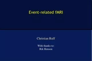
Auditory words every 20s Gamma functions ƒi() of peristimulus time (Orthogonalised) SPM{F} Sampled every TR = 1.7s Design matrix, X [x(t)ƒ1() | x(t)ƒ2() |...] … 0 time {secs} 30 General Linear Model in SPM
Overview 1. Block/epoch vs. event-related fMRI 2. (Dis)advantages of efMRI 3. GLM: Convolution 4. Temporal Basis Functions
Temporal basis functions • Fourier Set Windowed sines & cosines Any shape (up to frequency limit) Inference via F-test
Temporal basis functions • Finite Impulse Response Mini “timebins” (selective averaging) Any shape (up to bin-width) Inference via F-test
Temporal basis functions • Fourier Set / FIR Any shape (up to frequency limit / bin width) Inference via F-test • Gamma Functions Bounded, asymmetrical (like BOLD) Set of different lags Inference via F-test
Temporal basis functions • Fourier Set / FIR Any shape (up to frequency limit / bin width) Inference via F-test • Gamma Functions Bounded, asymmetrical (like BOLD) Set of different lags Inference via F-test • “Informed” Basis Set Best guess of canonical BOLD response Variability captured by Taylor expansion “Magnitude” inferences via t-test…?
Temporal basis functions “Informed” Basis Set (Friston et al. 1998) • Canonical HRF (2 gamma functions) Canonical
Temporal basis functions “Informed” Basis Set (Friston et al. 1998) • Canonical HRF (2 gamma functions) plus Multivariate Taylor expansion in: time (Temporal Derivative) Canonical Temporal
Temporal basis functions “Informed” Basis Set (Friston et al. 1998) • Canonical HRF (2 gamma functions) plus Multivariate Taylor expansion in: time (Temporal Derivative) width (Dispersion Derivative) Canonical Temporal Dispersion
Temporal basis functions “Informed” Basis Set (Friston et al. 1998) • Canonical HRF (2 gamma functions) plus Multivariate Taylor expansion in: time (Temporal Derivative) width (Dispersion Derivative) • “Magnitude” inferences via t-test on canonical parameters (providing canonical is a reasonable fit) Canonical Temporal Dispersion
Temporal basis functions “Informed” Basis Set (Friston et al. 1998) • Canonical HRF (2 gamma functions) plus Multivariate Taylor expansion in: time (Temporal Derivative) width (Dispersion Derivative) • “Magnitude” inferences via t-test on canonical parameters (providing canonical is a reasonable fit) • “Latency” inferences via tests on ratio of derivative: canonical parameters Canonical Temporal Dispersion
Other approaches (e.g., outside SPM) • Long Stimulus Onset Asychrony (SOA) • Can ignore overlap between responses (Cohen et al 1997) • … but long SOAs are less sensitive • Fully counterbalanced designs • Assume response overlap cancels (Saykin et al 1999) • Include fixation trials to “selectively average” response even at short SOA (Dale & Buckner, 1997) • … but often unbalanced, e.g. when events defined by subject • Define HRF from pilot scan on each subject • May capture inter-subject variability (Zarahn et al, 1997) • … but not interregional variability • Numerical fitting of highly parametrised response functions • Separate estimate of magnitude, latency, duration (Kruggel et al 1999) • … but computationally expensive for every voxel
Which temporal basis set? In this example (rapid motor response to faces, Henson et al, 2001)… Canonical + Temporal + Dispersion + FIR … canonical + temporal + dispersion derivatives appear sufficient to capture most activity … may not be true for more complex trials (e.g. stimulus-prolonged delay (>~2 s)-response) … but then such trials better modelled with separate neural components (i.e., activity no longer delta function) + constrained HRF (Zarahn, 1999)
Overview 1. Block/epoch vs. event-related fMRI 2. (Dis)advantages of efMRI 3. GLM: Convolution 4. BOLD impulse response 5. Temporal Basis Functions 6. Timing Issues
Timing issues: Sampling TR=4s Scans • Typical TR for 60 slice EPI at 3mm spacing is ~ 4s
Timing issues: Sampling TR=4s Scans • Typical TR for 48 slice EPI at 3mm spacing is ~ 4s • Sampling at [0,4,8,12…] post- stimulus may miss peak signal Stimulus (synchronous) SOA=8s Sampling rate=4s
Timing issues: Sampling TR=4s Scans • Typical TR for 48 slice EPI at 3mm spacing is ~ 4s • Sampling at [0,4,8,12…] post- stimulus may miss peak signal • Higher effective sampling by: 1. Asynchrony e.g., SOA=1.5TR Stimulus (asynchronous) SOA=6s Sampling rate=2s
Timing issues: Sampling TR=4s Scans • Typical TR for 48 slice EPI at 3mm spacing is ~ 4s • Sampling at [0,4,8,12…] post- stimulus may miss peak signal • Higher effective sampling by: 1. Asynchrony e.g., SOA=1.5TR2. Random Jitter e,g., SOA=(2±0.5)TR Stimulus (random jitter) Sampling rate=2s
Timing issues: Sampling TR=4s Scans • Typical TR for 48 slice EPI at 3mm spacing is ~ 4s • Sampling at [0,4,8,12…] post- stimulus may miss peak signal • Higher effective sampling by: 1. Asynchrony e.g., SOA=1.5TR2. Random Jitter e,g., SOA=(2±0.5)TR • Better response characterisation (Miezin et al, 2000) Stimulus (random jitter) Sampling rate=2s
T=16, TR=2s T0=16 o T0=9 o x2 x3 Scan 1 0 Timing issues: Slice-Timing T1 = 0 s T16 = 2 s
Bottom Slice Top Slice TR=3s SPM{t} SPM{t} Interpolated SPM{t} Derivative SPM{F} Timing issues: Slice-timing • “Slice-timing Problem”: Slices acquired at different times, yet model is the same for all slices different results (using canonical HRF) for different reference slices (slightly less problematic if middle slice is selected as reference, and with short TRs) • Solutions: 1. Temporal interpolation of data … but less good for longer TRs 2. More general basis set (e.g., with temporal derivatives) … but inferences via F-test
Overview 1. Block/epoch vs. event-related fMRI 2. (Dis)advantages of efMRI 3. GLM: Convolution 4. BOLD impulse response 5. Temporal Basis Functions 6. Timing Issues 7. Design Optimisation – “Efficiency”
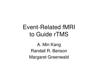
Design Efficiency • HRF can be viewed as a filter (Josephs & Henson, 1999) • We want to maximise the signal passed by this filter • Dominant frequency of canonical HRF is ~0.04 Hz The most efficient design is a sinusoidal modulation of neural activity with period ~24s • (e.g., boxcar with 12s on/ 12s off)
Sinusoidal modulation, f = 1/33s = = Stimulus (“Neural”) HRF Predicted Data A very “efficient” design!
Blocked, epoch = 20s Stimulus (“Neural”) HRF Predicted Data = = Blocked-epoch (with small SOA) quite “efficient”
Blocked (80s), SOAmin=4s, highpass filter = 1/120s = “Effective HRF” (after highpass filtering) (Josephs & Henson, 1999) = Stimulus (“Neural”) HRF Predicted Data Very ineffective: Don’t have long (>60s) blocks!
Randomised, SOAmin=4s, highpass filter = 1/120s = = Stimulus (“Neural”) HRF Predicted Data Randomised design spreads power over frequencies
Design efficiency • T-statistic for a given contrast: T = cTb / var(cTb) • For maximum T, we want minimum standard error of contrast estimates (var(cTb)) maximum precision • Var(cTb) = sqrt(2cT(XTX)-1c) (i.i.d) • If we assume that noise variance (2) is unaffected by changes in X, then our precision for given parameters is proportional to the design efficiency: e(c,X) = { cT (XTX)-1 c }-1 We can influence e (a priori) by the spacing and sequencing of epochs/events in our design matrix e is specific for a given contrast!