Download
1 / 20
200 likes | 267 Vues
Learn how to tie well logs to seismic events, load seismic data, estimate wavelets, and more in this comprehensive project setup guide.

E N D
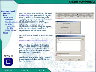
Create New Project • After the check shot correction shown in the Geoview part is completed, the logs need to be tied to the seismic events. Acoustic impedance corresponds to near offset reflectivity, while elastic impedance corresponds to far offset reflectivity. Hence will acoustic impedance be used for tying the logs to the near offset stack, and elastic impedance to the far offset stack. • The files needed can be downloaded from here: • http://www.ipt.ntnu.no/e-learning/seismics/ • Start the Elog module by clicking the ’Elog’ button in the Geoview window. You are getting prompted to select a project. Since this is the first project, a new one has to be created. • Toggle the ’Start a New Project’ option in the appearing window and fill out the form as shown.
Well_1 • Select ‘Well_1’ in the first appearing windown. The log suite of ‘Well_1’ should appear promptly in the main window of Elog.
Well_1 • We only want to display the density, p- and s-velocity in the Elog window for the further exercise. After the check shot correction, ‘P-wave_chk’ should be used as P-wave log instead of the previous ‘P-wave’. • Click on the eye-shaped button on the toolbar menu and click the ‘Logs’ folder to display only the ‘P-wave_chk’, ‘S-wave’ and ‘density’. Also change the ‘Start Amplitude’ and ‘End Amplitude’ for the density log as shown. • Make sure that the the ‘density’ log is the ‘Active’, or default, density log. Click on the ‘Active logs’ button and complete as shown. The ‘Ei/Vp’ log shows up under the density tag since this was assigned density when red from file.
Open Seismic from SEGY file • The near and far offset stack need to be loaded. Select the ‘From SEGY File’ option under ‘Seismic’ in the main window of Elog. • Add the ‘near.sgy’ and ‘far.sgy’ files as shown and click ‘Next’. • Since the UTM x and y are removed from the SEGY trace headers, CDP number is the primary key for assigning the traces to bin location. Toggle the options as shown to the right and click ‘Next’.
Open Seismic from SEGY file • For unknown reasons, the software is sometimes unable to read the trace sorting code and measurement system from the SEGY trace headers. Instead, the user gets prompted for this information. Assign this information as shown and click ‘Ok’. (Note that the default sample rate is micro seconds, not ms). • Click ‘Next’ on the two following windows.
Open Seismic from SEGY file • The geometry is defined in the next window and is assigned to both volumes. The CDP spacing is the same as cross-line spacing for this file. The value should be set to 25 m. • The origin is the position of the first CDP for a 2D line. • Click ‘Ok’ to complete the process. In the last window appearing, the well position is tied to CDP number. Assign Well_1 to CDP 37 and make sure that the ‘Used’ flag is shown in the ‘Usage’ column. • If the ‘Well to Seismic Map Menu’ does not appear, you can access it from the ‘Database’-option from the Strata main window. 25.00
Open Seismic from SEGY file • The near and far offset stack are now read into the database, appearing as volumes. As can be seen in the appearing window, the well is highly uncorrelated to the seismic data and the well needs to be shifted to match the strong peak. This peak is the top Cretaceous. • The seismic window can be closed.
Open Seismic from SEGY file • The log panel can easily be rearranged by clicking and dragging the log labels. • A portion of the near offset stack is automatically shown on the log panel. The red trace marks the well position.
Wavelet Estimation • Since the well is uncorrelated to the seismic data, the initial wavelet must be estimated from the seismic data alone, using a statistical least square approach. Don’t worry, the software will take care of this for you. • We start with correlation to the near offset stack and continue on with the far offset stack later. Select the ‘Statistical’ option under the ‘Wavelet’ menu as shown. • In the next window, the time and CDP range for wavelet extraction is assigned. The seismic data are muted above 2000 ms, and the well ends at approximately 2500 ms. The well was located at CDP 37, so selecting the neighboring traces from 25 to 45 should be appropriate. • Complete the form as show and hit ‘Next’. Also hit ‘Next’ on the following window.
Wavelet Estimation • The default wavelet length of 200 ms is way too long. Change this to 90 ms and click the ‘Next’ button for an initial try. • The extracted wavelet appears in a new window. Note that the text on the grey tab for this wavelet is colored red, meaning that this is now the ‘current’ wavelet, or the default wavelet used for generating synthetics.
Correlate – Near Offset • An initial shift of the well must be applied before the log can be stretched. • Click the correlate button in the Elog main window. Select the near volume as shown and click ‘Ok’. • Elog now computes a composite trace from the neighboring radius of 4 traces on the near volume. This trace is shown in red at the log panel. The blue trace also shown is computed from ‘Wave1’ and acoustic impedance, which in turn is computed from the active P-velocity and density. • The blue trace needs to be scaled down to correspond to the composite trace. This can be achieved by the display options. • Click the ‘eye’ button.
Correlate – Near Offset • Modify the seismic view from the display options as shown. The ‘trace excursion’ field is a scale factor multiplied to the blue and red trace. This should result in the log panel.
Correlate – Near Offset • At the base of the log panel is a field showing the zero lag cross correlation coefficient between the blue and red trace. Click on the ‘Parameters …’ button to modify the correlation window as shown. • Click the ‘Cross Correlation Plot’ button. The plot appearing suggests to shift the blue trace down. Also, due to the deviated path, it also needs to stretched.
Correlate – Near Offset • Obviously, the large peak on the blue trace corresponds to the nearest peak at the composite trace. Mark these peaks by clicking on them and apply the shift by clicking the ‘Stretch’ button at the base of the log panel. Note that the correlation coefficient hopefully increases. • By applying a stretch from only one pick shifts the logs. Picking more events stretches the logs.
Correlate – Near Offset • After the logs are shifted, a new wavelet can be estimated from a combination of the well log and seismic data. • Select the ‘Use Well’ option from the ‘Wavelet’ menu and estimate a new wavelet as shown. • Note that the blue trace gets automatically updated with the new wavelet. • The parameters shown here are only sample values. This process should be repeated with other values to obatin a better wavelet estimate.
Correlate – Near Offset • Due to the strongly deviated path, the log must be stretched. Pick events as shown and click the ‘Stretch’ button. This is more a trial and error exercise than science, and patience is probably an apropriate tool. After the stretch is applied, another wavelet can be estimated from the wells. This procedure is repeated until the synthetic • Matches the seismic properly. Click ‘Ok’ when done. • Save the corrected P-wave as shown below.
Correlate – Far Offset • Elastic impedance should be used for log correlation rather than acoustic impedance when correlating to far offset PP stacks. • There is yet no option for using elastic impedance for log correlation in Hampson-Russell, but this can be overcome as follows. • Click on the eye-button in the Elog window and go to the ‘Logs’ folder. Display only the P-wave log and ‘Ei/Vp’. • Click on the ‘Active logs’ button and select ‘Ei/Vp’ for density log. Multiplying this by the P-wave log in order to obtain acoustic impedance will instead yield elastic impedance, which in turn can be used for log correlation to far offset stack. • The elastic impedance log was generated in MatLab at 36 average angle of incidence and transmission, which is believed to correspond to the far offset stack.
Correlate – Far Offset • Click the ‘Correlate’ button in the main window and select the ‘far’ volume this time. • Extract a new wavelet from the well log and follow the same procedure for log correlation to the far offset stack as for the near offset stack. • Exit and save the correlated log as shown below.
Correlate – Far Offset • Back in the main window, select the ‘Display Seismic’ option from the ‘Seismic’ menu. The ‘far’ volume is displayed. • In the seismic window, click the ‘eye’ to get the display option and go to the ‘Insert’ folder. Select the ‘Synthetic Trace’ option from the upper pull-down menu as shown. Click ‘OK’ when done. A synthetic trace generated from the correlated logs and the current wavelet is displayed on the seismic (shown on the next slide).
Display Well Tie • The well tie is displayed as a red synthetic trace. • As probably noted, after correlation, a new P-wave log is created. For every such log, there is also created a time-table which is used for computing ‘tie-corrections’. This table is also applied to the other logs when displayed together. • Close all windows and save the project. Also agree to export the logs created during correlation to the database.