Understanding Power Functions & Higher Degree Polynomials: Analysis and Modeling Techniques
This guide covers the fundamentals of power functions and higher-degree polynomials, exploring their forms, properties, and analyses. A power function is defined as ( f(x) = kx^a ) where both ( k ) and ( a ) are non-zero constants. The document discusses essential concepts like domain, range, continuity, symmetry (even/odd functions), boundedness, local extrema, asymptotes, and end behavior. It includes examples to illustrate how to analyze graphs and find zeros, multiplicity of roots, and sketch corresponding graphs.

Understanding Power Functions & Higher Degree Polynomials: Analysis and Modeling Techniques
E N D
Presentation Transcript
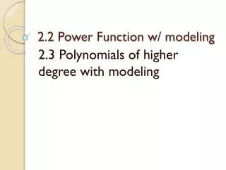
2.2 Power Function w/ modeling 2.3 Polynomials of higher degree with modeling
Power function • A power function is any function that can be written in the form: f(x) = kxa, where k and a ≠ 0 • Monomial functions: f(x) = k or f(x) = kxn • Cubing function: f(x) = x3 • Square root function: f(x) = x • Higher degree: (standard form) p(x) = anxn + an-1xn-1 + an-2xn-2 +… + a1x + a0
Analyzing Power functions • To do you will find the following: domain range continuous/discontinuous increasing/decreasing intervals even (symmetric over y-axis)/odd function (symmetric over origin) boundedness local extrema (max/min) asymptotes (both VA and HA) end behavior (as it approaches both -∞ & ∞
Example: analyze f(x) = 2x4 • Power: 4, constant: 2 • Domain: (-∞,∞) • Range: [0, ∞) • Continuous • Increasing: [0,∞), decreasing: (-∞, 0] • Even: symmetric w/ respect to y-axis • Bounded below • Local minimum: (0, 0) • Asymptotes: none • End behavior: lim 2x4 = ∞, lim 2x4 = ∞ x -∞ x ∞ (in other words, on the left the graph goes up, on the right the graph goes up) Try one: f(x) = 5x3
Investigating end behavior • When determining end behavior you need to determine if the graph is going to -∞ (down) or ∞ (up) as x -∞ & as x ∞ • Example: graph each function in the window [-5, 5] by [-15, 15] . Describe the end behavior using lim f(x) & lim f(x) x -∞ x ∞ • f(x)=x3+2x2-5x-6: -∞,∞ • Do exploration
Finding 0’s • Find the 0’s of f(x) = 3x3 – x2 -2x • Algebraically: factor 3x3 – x2 -2x = 0 x(3x2 – x -2) = 0 x(3x + 2)(x - 1) = 0 x = 0, 3x + 2 = 0, x – 1= 0 x = 0, x = -2/3, x = 1 • Graphically: graph & find the 0’s (2nd trace #2)
Zeros of Polynomial function • Multiplicity of a Zero If f is a polynomial function and (x-c)m is a factor of f but (x – c)m+1 is not, then c is a zero of multiplicity m of f. • Zero of Odd and Even Multiplicity: If a poly. funct. f has a real 0 c of odd multiplicity, then the graph of f crosses the x-axis at (c, 0) & the value of f changes sign at x=c if a poly. funct. f has a real 0 c of even multiplicity, then the graph doesn’t cross the x-axis at (c, 0) & the value of f doesn’t change sign at x=0
Multiplicity • State the degree, list the 0’s, state the multiplicity of each 0 and what the graph does at each corresponding 0. then sketch the graph by hand (look at exponents: if 1 then crosses, if odd then wiggles, if even then tangent) • Examples: 1)f(x) = x2 + 2x – 8 degree: 2, 0’s: 2, -4, graph: crosses at x=-4 & x= 2 2) f(x) = (x + 2)3(x-1)(x-3)2 Now finish paper
Writing the functions given 0’s • 0, -2, 5 1) rewrite w/ a variable & opposite sign: x(x + 2)(x – 5) 2) simplify x(x2 -3x + -10) x3 – 3x2 – 10x Try one: -6, -4, 5
Homework: • p. 182 #, 28, 29 • p. 193-194 #2-6 even, 25-28 all, 34-38 even, 39-42 all, 49-52 all, 53, 54

![Data Modeling [Comparison of data modeling techniques ]](https://cdn0.slideserve.com/205866/data-modeling-comparison-of-data-modeling-techniques-dt.jpg)