Download
1 / 33
330 likes | 348 Vues
Learn about probabilistic forecasts & ensemble prediction for more reliable weather forecasts. Discover methods to evaluate forecast reliability, sharpness, & spread-error relationships. Benefits & dangers of ensemble averaging explained.

E N D
NOAA Earth System Research Laboratory A primer on ensemble weather prediction and the use of probabilistic forecasts Tom Hamill NOAA Earth System Research Laboratory Physical Sciences Division tom.hamill@noaa.gov Presentation to 2011 Albany Utility Wind Integration Workshop
Uncertainty is inevitable, and“state dependent” The Lorenz (1963) model σ, ρ, βare fixed. A toy dynamical system that illustrates the problem of “deterministic chaos” that we encounter in weather prediction models. Forecast uncertainty grows more quickly for some initial conditions than others. from Tim Palmer’s chapter in 2006 book “Predictability of Weather and Climate”
Amount of uncertainty depends on weather regime. Lower wind uncertainty; no major weather systems around. High wind uncertainty; timing & strength of trough.
Forecast uncertainty also contributed by model imperfections “Parameterizations” Much of the weather occurs at scales smaller than those resolved by the weather forecast model. A forecast model must treat, or “parameterize” the effects of the sub-gridscale on the resolved scale. Problems: (1) no variability at scales smaller than the box from this model; (2) parameterizations are approximations, and often not good ones.
“Ensemble prediction” Perhaps different forecast models, or built-in stochastic effects to account for model uncertainty
Desirable properties ofprobabilistic forecasts & common methods to evaluate them. • Reliability/calibration: when you say X%, it will happen X% of the time. • calibration: observed and ensemble considered samples from the same probability distribution • Specificity of the forecast, i.e., sharpness. Deviations from the climatological. We want forecasts as sharp as they can be as long as they’re reliable.
Reliability diagrams Curve tells you what the observed frequency was each time you forecast a given probability. This curve ought to lie along y = x line. Here this shows the ensemble-forecast system over-forecasts the probability of light rain. Ref: Wilks text, Statistical Methods in the Atmospheric Sciences
Inset histogram tells you how frequently each probability was issued. Perfectly sharp: frequency of usage populates only 0% and 100%. Reliability diagrams Ref: Wilks text, Statistical Methods in the Atmospheric Sciences
BSS = Brier Skill Score Reliability diagrams BS(•) measures the Brier Score, which you can think of as the squared error of a probabilistic forecast. Perfect: BSS = 1.0 Climatology: BSS = 0.0 Ref: Wilks text, Statistical Methods in the Atmospheric Sciences
Sharpness “Sharpness” measures the specificity of the probabilistic forecast. Given two reliable forecast systems, the one producing the sharper forecasts is preferable. Might be measured with standard deviation of ensemble about its mean. But: don’t want sharp if not reliable. Implies unrealistic confidence.
“Spread-error”relationshipsare important, too. Small-spread ensemble forecasts should have less ensemble-mean error than large-spread forecasts, in some sense a conditional reliability dependent upon amount of sharpness. ensemble-mean error from a sample of this pdf on avg. should be low. ensemble-mean error should be moderate on avg. ensemble-mean error should be large on avg.
General benefits from use of ensembles • Averaging of many forecasts reduces error. • Proper use of probabilistic information permits better decisions to be made based on risk tolerance.
Dangers of “ensemble averaging”(smoothes out meteorological features) individual members decision threshold wind speed Here the ensemble tells you something useful… a wind ramp is coming, but the exact timing is uncertain. Information lost if you boil it down to its average. time ensemble average decision threshold wind speed time
Two general methods of providing you with useful local probabilistic information • Dynamical downscaling (run high-resolution ensemble systems to provide local detail). • Statistical downscaling (post-process coarser resolution model to fill in the local detail and missing time scales).
Potential value of dynamic downscaling An example from high-resolution ensembles run during the NSSL-SPC Hazardous Weather Test Bed, forecast initialized 20 May 2010 http://tinyurl.com/2ftbvgs 32-km SREF P > 0.5” 4-km SSEF P > 0.5 “ Verification With warm-season precipitation, coarse resolution and parameterized convection of operational SREF clearly is inferior to the 4-km, resolved convection in SSEF.
We still have a way to go to provide sharp, reliable forecasts directly from hi-res. ensembles. Case: Arkansas floods An example from NSSL-SPC Hazardous Weather Test Bed, forecast initialized 10 June 2010 http://tinyurl.com/34568hp SREF P > 2.0” 4-km SSEF P > 2.0 “ Verification (radar QPE) A less than 30% probability of > 2 inches rainfall from SSEF, while better than SREF, probably does not set off alarm bells in forecasters’ heads.
Statistical downscaling • Direct probabilistic forecasts from a global model may be unreliable, and perhaps too coarse time granularity for your purposes (winds every 3 h). • Assume you have: • a long time series of wind measurements. • a long time series of forecasts from a fixed model that hasn’t changed (“reforecasts”) • Can correct for discrepancies between forecast and observed using past data, adjust today’s forecast, quantify uncertainty. • Proven technique in “MOS” – what’s new here is the especially long time series of ensemble forecasts, helpful for making statistical adjustments in long-lead and rare events.
Potential value of statistical downscaling using “reforecasts” Post-processing with large training data set can permit small-scale detail to be inferred from large-scale, coarse model fields.
An example of a statistical correction technique using those reforecasts Today’s forecast (& observed) For each pair (e.g. red box), on the left are old forecasts that are somewhat similar to this day’s ensemble-mean forecast. The boxed data on the right, the analyzed precipitation for the same dates as the chosen analog forecasts, can be used to statistically adjust and downscale the forecast. Analog approaches like this may be particularly useful for hydrologic ensemble applications, where an ensemble of weather realizations is needed as inputs to a hydrologic ensemble streamflow system.
A next-generation reforecast • Model: NCEP GFS ensemble that will be operational later in 2011. • Reforecast: at 00Z, compute full 10-member forecast, every day, for last 30 years out to 16 days. • Continue to generate real-time forecasts with this model for next ~5 years. • Reforecasts computed by late 2011. • More details in supplementary slides.
Making reforecast dataavailable to you • Store 130 TB (fast access) of “important” agreed-upon subset of data. • Will design software to serve this out to you in several manners (http, ftp, OPeNDAP, etc.). • Archive full 00Z reforecasts and initial conditions ~=778 TB. DOE expected to store this for us (slow access).
Expected fields in the “fast” archive • Mean and every member • For wind energy, 10-m and 80 m winds, 80-m wind power. • 3-hourly out to 72h, then 6-hourly thereafter. • Lots of other data (details in backup slides)
Conclusions • Ensembles may provide significant value-added information to you. • I’m interested in talking with you more to understand how ensembles information (especially reforecasts) can be tailored to help with your decision making.
Expected fields we’ll save in the reforecast “fast” archive • Mandatory level data: • Geopotential height, temperature, u, v, at 1000, 925, 850, 700, 500, 300, 250, 200, 100, 50, and 10 hPa. • Specific humidity at 1000, 925, 850, 700, 500, 300, 250, 200 • PV (K m2 kg-1 s-1 ) on θ = 320K surface. • Wind components, potential temperature on 2 PVU surface.
Fixed fields to save once • field capacity • wilting point • land-sea mask • terrain height
Proposed single-level fields for “fast” archive • Surface pressure (Pa) • Sea-level pressure (Pa) • Surface (2-m) temperature (K) • Skin temperature (K) • Maximum temperature since last storage time (K) • Minimum temperature since last storage time (K) • Soil temperature (0-10 cm; K) • Volumetric soil moisture content (proportion, 0-10 cm) – • Total accumulated precipitation since beginning of integration (kg/m2) • Precipitable water (kg/m2, vapor only, no condensate) • Specific humidity at 2-m AGL (kg/kg; instantaneous) – • Water equivalent of accumulated snow depth (kg/m2) – • CAPE (J/kg) • CIN (J/kg) • Total cloud cover (%) • 10-m u- and v-wind component (m/s) • 80-m u- and v-wind component (m/s) • Sunshine duration (min) • Snow depth water equivalent (kg/m2) • Runoff • Solid precipitation • Liquid precipitation • Vertical velocity (850 hPa) • Geopotential height of surface • Wind power (=windspeed3 at 80 m*density)
Proposed fields for “fast” archive • Fluxes (W/m2 ; average since last archive time) • sensible heat net flux at surface • latent heat net flux at surface • downward long-wave radiation flux at surface • upward long-wave radiation flux at surface • upward short-wave radiation at surface • downward short-wave radiation flux at surface • upward long-wave radiation at nominal top • ground heat flux.
Uncalibratedensemble? Here, the observed is outside of the range of the ensemble, which was sampled from the pdf shown. Is this a sign of a poor ensemble forecast?
Uncalibratedensemble? You just don’t know…it’s only one sample You just don’t know; it’s only one sample. Here, the observed is outside of the range of the ensemble, which was sampled from the pdf shown. Is this a sign of a poor ensemble forecast?
Rank 1 of 21 Rank 14 of 21 Rank 5 of 21 Rank 3 of 21
Rank histograms With lots of samples from many situations, can evaluate the characteristics of the ensemble. Happens when observed is indistinguishable from any other member of the ensemble. Ensemble hopefully is reliable. Happens when observed too commonly is lower than the ensemble members. Happens when there are either some low and some high biases, or when the ensemble doesn’t spread out enough. ref: Hamill, MWR, March 2001