Download
1 / 49
490 likes | 521 Vues
Understand complexities, differences between BFS and DFS, Dijkstra's Algorithm for pathfinding, and priority queue utilization in graph traversals. Dive into path lengths, tree constructions, and algorithmic complexities.

E N D
Shortest Paths • Distance is the length of the shortest path between two nodes • Breadth-first search (BFS) creates one BFS tree rooted at the initial node • Just one tree since we only care about nodes connected to the initial node. The rest have infinite distance. • BFS tree is a shortest path tree • Distance is the tree depth where each node resides • Complexity? – Examine algorithm CS 312 – Graph Algorithms - Paths
Careful look at BFS Complexity • Initialization step is O(|V|) • Complexity of main section? • Each v considered exactly twice (one eject and one inject) • Must consider what the complexity is of eject and inject • For each v, each edge is considered exactly once for directed graphs and twice for undirected graphs • O(|V|*complexity(inject) + |V|*complexity(eject) + (1 or 2)*|E|) = ? CS 312 – Graph Algorithms - Paths
Careful look at BFS Complexity • Complexity of main section? • Each v considered exactly once (one eject and one inject) • Must consider what the complexity is of eject and inject • For each v, each edge is considered exactly once for directed graphs and twice for undirected graphs • O(|V|*complexity(inject) + |V|*complexity(eject) + (1 or 2)*|E|) = ? • For a simple queue the complexity of inject and eject are O(1) • Note that since we start at just one node and consider all reachable nodes Vr, the number of unique reachable edges Er lies between Vr-1 and 2Vr2 and thus Er = Ω(Vr) (i.e. in complexity sense Er≥Vr) • O(|Er|) = O(|E|) • Thus total main section complexity is O(|E|) • Total overall is O(|V|+|E|) CS 312 – Graph Algorithms - Paths
DFS and BFS Comparisons • DFS (e.g. Explore(G,v)) goes as deep as it can before backtracking for other options • Typically will not find shortest path • Could find a goal deep in the search tree relatively fast • Only need memory equal to stack depth • Infinitely deep paths can get you stuck • BFS • Guaranteed to find shortest path • Is that always important? • Memory will be as wide as the search tree (grows exponentially) • Long search if goal is deep in the search tree • “Best” First Search/Intelligent Search - Later CS 312 – Graph Algorithms - Paths
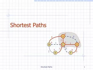
Lengths on Edges a 6 s 1 b 2 • Often edges will correspond to different lengths • Map • Path cost, time, distance, reward, negative values, etc. • Each eE has le, also written for u,v as l(u,v) or luv • How do we find shortest path in this case • Assume positive edge lengths for the moment • Dijkstra’s algorithm • Replace BFS simple queue with a Priority Queue • Priority queue keeps node with smallest current distance at front • Update appropriate distances after a new node is opened • Arriving at a visited node may actually shorten the path • You will use Dijkstra’s in your “Network Routing” project CS 312 – Graph Algorithms - Paths
Priority Queue Operations • Maintains a set of elements each with an associated numeric key (e.g. distance) • We will review complexity details in a bit • Following are four operations which we will consider CS 312 – Graph Algorithms - Paths
Dijkstra’s Algorithm a 6 s 1 b 2 CS 312 – Graph Algorithms - Paths
Dijkstra Example Length of shortest paths: A: 0 B: ∞ C: ∞ D: ∞ E: ∞ H = makequeue(V) Priority Queue H: A:0, B:∞, C:∞, D:∞, E:∞ CS 312 – Graph Algorithms - Paths
Dijkstra Example Length of shortest paths: A: 0 B: 4 C: 2 D: ∞ E: ∞ Pull A off of H Priority Queue H: C:2, B:4, D:∞, E:∞ CS 312 – Graph Algorithms - Paths
Dijkstra Example Length of shortest paths: A: 0 B: 3 C: 2 D: 6 E: 7 Pull C off of H and update Priority Queue H: B:3, D:6, E:7 B changes it prev pointer from A to C Note that once you dequeue a node (deletemin) you are guaranteed that that there is no shorter path to that node. Why?
Dijkstra Example Length of shortest paths: A: 0 B: 3 C: 2 D: 5 E: 6 Pull B off of H and update Priority Queue H: D:5, E:6 Note that decreasekey just works on the frontier, ordering which are the best next nodes to expand, but never undermining an already expanded path
Dijkstra Example Length of shortest paths: A: 0 B: 3 C: 2 D: 5 E: 6 Pull D off of H and update and then E off of H Priority Queue H: E:6 CS 312 – Graph Algorithms - Paths
Dijkstra Example A: 0 B: 3 C: 2 D: 5 E: 6 Final Shortest Path Tree Constructed using prev(u) CS 312 – Graph Algorithms - Paths
**Challenge** Dijkstra’s Algorithm Complexity Give complete complexity in terms of V, E, and queue operations – assume makequeue just uses insert CS 312 – Graph Algorithms - Paths
Dijkstra Algorithm Complexity • Similar to BFS (O(|V| + |E|), but now we have a priority queue instead of a normal queue • Thus complexity will be O(|V|×(complexity of priority queue operations)+|E|×(complexity of priority queue operations)) • Different priority queue implementations have different complexities • Basic operations are insert, make-queue, decrease-key, and delete-min • For Dijkstra’s algorithm make-queue is done just once and is at least O(|V|). Worst case is O(|V|×(complexity of insert)) • delete-min is called once for every node |V| • decrease-key is called up to once for every edge |E| = |V|×Eavg • the overall complexity is: O(|V|×(insert) + |V|×(delete-min) + |E|×(decrease-key)) CS 312 – Graph Algorithms - Paths
Priority Queue (PQ) Implementations • Array • An array of size |V| • Indexed by node number, the key is the array element value • Decrease-key/Insert is O(1) • Delete-min is O(|V|) since need to search through entire array each time for smallest key • Can keep count of queue items to know when queue is empty, etc. • Dykstra Complexity with array PQ? • O(|V|×(insert) + |V|×(delete-min) + |E|×(decrease-key)) • An optimal implementation if graph is dense • Dense graphs are less common for large applications • Can we do better if sparse? CS 312 – Graph Algorithms - Paths
Priority Queue Implementations • D-ary Heap • Complete D-ary tree (binary common) • Special Constraint: The key value of any node of the tree is less than or equal to that of its children • Thus the minimum node is always at the top of the tree • Insert: CS 312 – Graph Algorithms - Paths
Priority Queue Implementations • D-ary Heap • Complete D-ary tree (binary common) • Special Constraint: The key value of any node of the tree is less than or equal to that of its children • Thus the minimum node is always at the top of the tree • Insert: Put new key at next available tree spot (bottom rightmost). Let it "bubble up" tree path, swapping with the node above, until it gets to its proper spot. logdn time to "bubble up" • Delete-min: CS 312 – Graph Algorithms - Paths
Priority Queue Implementations • D-ary Heap • Complete D-ary tree (binary common) • Special Constraint: The key value of any node of the tree is less than or equal to that of its children • Thus the minimum node is always at the top of the tree • Insert: Put new key at next available tree spot (bottom rightmost). Let it "bubble up" tree path, swapping with the node above, until it gets to its proper spot. logdn time to "bubble up" • Delete-min: Pulls off top and replaces it with last (rightmost) node of tree and then "sift down" (with smallest) to its proper spot – dlogdn time to "sift down" since have to sort on d sub-nodes at each level to find min to bring up, note that total is O(logn) once we set d • Decrease-key: CS 312 – Graph Algorithms - Paths
Priority Queue Implementations • D-ary Heap • Complete D-ary tree (binary common) • Special Constraint: The key value of any node of the tree is less than or equal to that of its children • Thus the minimum node is always at the top of the tree • Insert: Put new key at next available tree spot (bottom rightmost). Let it "bubble up" tree path, swapping with the node above, until it gets to its proper spot. logdn time to "bubble up" • Delete-min: Pulls off top and replaces it with last (rightmost) node of tree and then "sift down" (with smallest) to its proper spot – dlogdn time to "sift down" since have to sort on d sub-nodes at each level to find min to bring up, note that total is O(logn) once we set d • Decrease-key: same "bubble-up" as Insert, logd(n) if maintain separate index into the heap to get to the right element, else O(n) • More on this in a second CS 312 – Graph Algorithms - Paths
Priority Queue Implementations • Binary Heap Implementation notes (can use for project) • Can implement the D-ary heap with an array • Note this is not an array implementation of a priority queue • A balanced binary tree has a simple fast array indexing scheme CS 312 – Graph Algorithms - Paths
Priority Queue Implementations • Binary Heap Implementation notes (can use for project) • Can implement the binary heap with an array • Note this is not an array implementation of a priority queue • A balanced binary tree has a simple fast array indexing scheme • node j has parent floor(j/2) • node j has children 2j and 2j+1 • How do you find an arbitrary node to do decrease_key? – As is, it would be O(|V|) to find the node, thus messing up overall complexity • Can keep a separate array of size |V| which points into the binary heap for each node, thus allowing O(1) lookup of an arbitrary node • Each time you do a binary heap operation with a change in the heap, you need to adjust the pointers in the pointer array. CS 312 – Graph Algorithms - Paths
PQ Implementation Example 4 7 1 2 1 2 3 3 6 5 4 5 7 6 Pointer Array Binary Heap Array Note the indexes in the graph and tree are different Assume we insert nodes 2-6 into the PQ all with initial key of ∞ – what will it look like? CS 312 – Graph Algorithms - Paths
PQ Implementation Example 2:∞ 4 7 1 3:∞ 2 4:∞ 1 2 3 3 5:∞ nil 6:∞ 6 nil 5 4 5 7 6 Pointer Array Binary Heap Array HC: 5 Note the indexes in the graph and tree are different Assume we insert nodes 2-6 into the PQ – what will it look like? What happens if we call DecreaseKey(3,12)? CS 312 – Graph Algorithms - Paths
PQ Implementation Example 3:12 4 7 1 2:∞ 2 4:∞ 1 2 3 3 5:∞ nil 6:∞ 6 nil 5 4 5 7 6 Pointer Array Binary Heap Array HC: 5 Note the indexes in the graph and tree are different Assume we insert nodes 2-6 into the PQ – what will it look like? What happens if we call DecreaseKey(3,12)? What about Insert(1,15)? CS 312 – Graph Algorithms - Paths
PQ Implementation Example 3:12 4 7 1 2:∞ 2 1:15 1 2 3 3 5:∞ nil 6:∞ 6 4:∞ 5 4 5 7 6 Pointer Array Binary Heap Array HC: 6 Note the indexes in the graph and tree are different Assume we insert nodes 2-6 into the PQ – what will it look like? What happens if we call DecreaseKey(3,12)? What about Insert(1,15)? What about DM()? CS 312 – Graph Algorithms - Paths
PQ Implementation Example 1:15 4 7 1 2:∞ 2 4:∞ 1 2 3 3 5:∞ nil 6:∞ 6 nil 5 4 5 7 6 Pointer Array Binary Heap Array HC: 5 Note the indexes in the graph and tree are different Assume we insert nodes 2-6 into the PQ – what will it look like? What happens if we call DecreaseKey(3,12)? What about Insert(1,15)? What about DM()? CS 312 – Graph Algorithms - Paths
Dijkstra Algorithm Complexity • If dense then unsorted array implementation is best – why? • Binary heap better as soon as |E| < |V|2/log|V| • D-ary heap – depth of heap is logd|V| • constant factor improvement (log2d on depth), though deletemin is bit longer, since have to sort on d sub-nodes at each level to find min to bring up • Optimal balance is d ≈ |E|/|V| the average degree of the graph • Fibonacci heap – complex data structure makes this less appealing • O(1) (amortized) means over course of the algorithm average is O(1) • Data Structures Matter! CS 312 – Graph Algorithms - Paths
Network Routing Project • Interface, etc. is supplied. You will implement Dijkstra's with two different priority queue implementations: Array and D-ary Heap • binary is fine for the heap if you want • Hint: Implement and test first with simple array PQ implementation • Network routing uses Dijkstra’s algorithm to find the optimal (least-cost) path between a source and all other nodes • You select number of nodes and seed, and a random cost matrix is generated. • You will always find the distance from source to every node in the graph • Once you have generated the full routing table at a node you do not need to re-calculate paths each time • However, networks are constantly changing (new nodes, outages, etc.) so can recalculate each time • Just finding the best path from the source to the destination can be more efficient than finding them all, though same Big-O complexity • We used to have you do All-paths and One-path CS 312 – Graph Algorithms - Paths
Dijkstra Flow with Insert and Goal While Queue not empty u = deletemin() if u= g then break() for each edge (u,v) if dist(v) = ∞ (i.e. not visited ) insert(v, dist(u)+len(u,v)) prev(v) = u else if dist(v) > dist(u) + len(u,v) dist(v) = dist(u) + len(u,v) decreasekey(v, dist(u) + len(u,v)) prev(v) = u s g • If graph is large we do not need to start with all nodes in the queue • This is just a variant (subset) of the algorithm in the text • All-Paths vs One-path (my names) • All distances initially set to ∞ (which is also a flag for not yet queued) • Yellow: in the Queue • Red: removed from the Queue CS 312 – Graph Algorithms - Paths
Dijkstra Flow with Insert and Goal While Queue not empty u = deletemin() if u= g then break() for each edge (u,v) if dist(v) = ∞ (i.e. not visited ) insert(v, dist(u)+len(u,v)) prev(v) = u else if dist(v) > dist(u) + len(u,v) dist(v) = dist(u) + len(u,v) decreasekey(v, dist(u) + len(u,v)) prev(v) = u s g Yellow: in the Queue Red node: removed from Queue Red lines: current backpointers which create the cheapest path tree, they can only be created/updated with a just removed node CS 312 – Graph Algorithms - Paths
Dijkstra Flow with Insert and Goal While Queue not empty u = deletemin() if u= g then break() for each edge (u,v) if dist(v) = ∞ (i.e. not visited ) insert(v, dist(u)+len(u,v)) prev(v) = u else if dist(v) > dist(u) + len(u,v) dist(v) = dist(u) + len(u,v) decreasekey(v, dist(u) + len(u,v)) prev(v) = u s g Updated w/ decreasekey Next deletemin is minimal yellow node (those queued) No sense of direction towards g, just pushes out the shortest/cheapest frontier until g is finally reached decreasekey only an option when a removed node has an edge to a node already on the queue CS 312 – Graph Algorithms - Paths
Dijkstra Flow with Insert and Goal While Queue not empty u = deletemin() if u= g then break() for each edge (u,v) if dist(v) = ∞ (i.e. not visited ) insert(v, dist(u)+len(u,v)) prev(v) = u else if dist(v) > dist(u) + len(u,v) dist(v) = dist(u) + len(u,v) decreasekey(v, dist(u) + len(u,v)) prev(v) = u s g Why don't we need to revisit a note if it has been removed? If it is removed it is already on the least cost path and can never be modified. A later node could have an edge to a removed node but it would have to be a longer path (unless there were negative paths) CS 312 – Graph Algorithms - Paths
Dijkstra Flow with Insert and Goal While Queue not empty u = deletemin() if u= g then break() for each edge (u,v) if dist(v) = ∞ (i.e. not visited ) insert(v, dist(u)+len(u,v)) prev(v) = u else if dist(v) > dist(u) + len(u,v) dist(v) = dist(u) + len(u,v) decreasekey(v, dist(u) + len(u,v)) prev(v) = u s g We can't terminate just when g gets on the queue, but as soon as g is removed, then we know we have the shortest path CS 312 – Graph Algorithms - Paths
Dijkstra Flow with Insert and Goal While Queue not empty u = deletemin() if u= g then break() for each edge (u,v) if dist(v) = ∞ (i.e. not visited ) insert(v, dist(u)+len(u,v)) prev(v) = u else if dist(v) > dist(u) + len(u,v) dist(v) = dist(u) + len(u,v) decreasekey(v, dist(u) + len(u,v)) prev(v) = u g s Another decreasekey example CS 312 – Graph Algorithms - Paths
Dijkstra Flow with Insert and Goal While Queue not empty u = deletemin() if u= g then break() for each edge (u,v) if dist(v) = ∞ (i.e. not visited ) insert(v, dist(u)+len(u,v)) prev(v) = u else if dist(v) > dist(u) + len(u,v) dist(v) = dist(u) + len(u,v) decreasekey(v, dist(u) + len(u,v)) prev(v) = u s g Since g had the minimal key it is removed and we can terminate Note the red edges are the cheapest path tree from s Could continue and fill out the entire reachable graph, but not necessary since we reached the goal node CS 312 – Graph Algorithms - Paths
Complexity for One-path Dijkstra • Same as standard Dijkstra complexity? For typical cases • O(|V|×(insert) + |V|×(delete-min) + |E|×(decrease-key)) = O((|V|+|E|)log|V|) • Which should have better constants? • However, • In the main body of One-Path O(|V|) ≤ O(|E|) since it only considers reachable nodes, thus the main body is O(|E|log|V|) • Which is also the case for All-paths • One-path does not need to insert all nodes like All-paths, thus not needing the separate O(|V|log|V|) complexity (which can dominate in the rare cases where there are many nodes with 0 degree – no edges). Note we could just do all-paths and break when g is dequeued, which is an improvement, but still requires full queue creation. Note that if the break statement were dropped from One-path, the result would be the same as All-paths. • One-path still needs to initiate all node distances to ∞ but that is O(1) for each v leading to a full complexity of O(|V|+|E|log|V|) • All-paths also has to initiate node distances to ∞, but that O|V|) complexity is subsumed by the O(|V|log|V|) insert complexity. CS 312 – Graph Algorithms - Paths
Negative Edges a 3 s -2 b 4 • With negative edges we can't keep a guaranteed cheapest frontier, since each time we encounter a negative edge we would have to propagate back decreased costs • We won’t use a priority queue since we can’t guarantee the true shortest path is at the front anyway • Note that the maximum edges in a cheapest path is |V|-1, assuming there are no negative cycles • Just update all edges |V|-1 times (max possible path length) • Or until no changes are made • Gives opportunity for all negative edges in path to properly sum • All possible shorter path updates are given a chance (i.e. nodes are not pulled off the queue when they would have been if no negative paths) CS 312 – Graph Algorithms - Paths
Column c contains the shortest path lengths from S to node x comprising ≤ c edges
**Challenge ** Fill out rest of the table Complexity? Propose some shortcuts that would make the alg faster Do your shortcuts improve big-O? Column c contains the shortest path lengths from S to node x comprising ≤ c edges
Column c contains the shortest path lengths from S to node x comprising ≤ c edges
Known as the Bellman-Ford Algorithm Complexity is ? CS 312 – Graph Algorithms - Paths
Bellman-Ford Algorithm Complexity is |V|·|E| CS 312 – Graph Algorithms - Paths
Negative Cycles When there are negative cycles then by definition cheapest paths do not exist. CS 312 – Graph Algorithms - Paths
Negative Cycles When there are negative cycles then by definition cheapest paths do not exist. Run Bellman-Ford one more iteration (|V| times). There is a negative cycle iff any cheapest path (distance value) decreases again CS 312 – Graph Algorithms - Paths
Shortest Path with DAGs c 4 a 2 -3 s 2 d b 6 -1 Negative paths are all right since there are no cycles and the linearization will cause appropriate ordering Complexity? CS 312 – Graph Algorithms - Paths
Graph Paths Conclusion • With Breadth First Search (bfs) algorithms we have found efficient ways to find shortest paths in different types of graphs • Non-weighted edges – simple bfs • Weighted edges – Dijkstra's • Negative edges – Bellman-Ford • DAGs – Dag-shortest-path() • Efficiency for some of these can be strongly effected by choice of data structure implementation CS 312 – Graph Algorithms - Paths