
Data Quality Data Exploration
E N D
Presentation Transcript
Data QualityData Exploration CSC 576: Data Mining
Today • Data Quality • Data Exploration
Data Quality Report • A data quality report includes tabular reports that describe the characteristics of each feature in a dataset using standard statistical measures of central tendencyand variation. • In KNA textbook, ABT refers to “Analytics Base Table” • The tabular reports are accompanied by data visualizations: • histogramfor each continuous feature • bar plotfor each categorical feature • also generally used for continuous features with cardinality < 10
Tabular Structure in a Data Quality Report • Card = Cardinality • Measures the number of distinct values present for a feature Note the differences between each table.
Data Exploration: Getting to Know the Data • For categorical features: • Examine the mode, 2nd mode, mode %, and 2nd mode % • Represent the most common levels within these features • Will identify if any levels dominate the dataset. • For continuous features: • Examine the mean and standard deviation of each feature • Get a sense of the central tendency and variation of the values • Examine the minimum and maximum values to understand the range that is possible for each feature • Histograms of continuous features will resemble the following well understood shapes (probability distributions) • Recognizing the distribution of values for a feature will be useful when applying machine learning models
Uniform Distribution Sometimes indicative of a feature such as an ID, rather than something more interesting • A uniform distribution indicates that a feature is equally likely to take a value in any of the ranges present.
Naturaly occurring phenomena (heights, weights of a randomly selected group of men, women) tend to follow a normal distribution. Normal Distribution • Features following a normal distribution are characterized by a strong tendency towards a central value and symmetrical variation to either side of this. • Unimodal:single peak around the central tendency
Skewed Distributions • Skew is simply a tendency towards very high (right skew) or very low (left skew) values.
Exponential Distribution Examples: number of times a person has been married; number of times a person has made an insurance claim • In a feature following an exponential distribution the likelihood of occurrence of a small number of low values is very high, but sharply diminishes as values increase.
Example: measure of heights of a randomly selected group of Irish men and women Multimodal Distribution • A feature characterized by a multimodal distribution has two or more very commonly occurring ranges of values that are clearly separated. • Bi-modal distribution: two clear peaks • “two normal distributions pushed together” • Tends to occur when a feature contains a measurement made across two distinct groups
Normal Distribution • The probability density function for the normaldistribution (or Gaussian distribution) is • x is any value • μ (mu) and σ (sigma) are parameters that define the shape of the distribution • the population mean and population standard deviation
68-95-99.7 Rule • The 68 − 95 − 99.7 rule is a useful characteristic of the normal distribution. • The rule states that approximately: • 68% of the observations will be within oneσ of μ • 95% of observations will be within twoσ of μ • 99.7% of observations will be within threeσ of μ. Very low probability of observations occurring that differ from the mean by more than two standard deviations.
Case Study • Become familiar with the central tendency and variation of each feature using the data quality report. • Note bar graphs and histograms (earlier slides). • Note number of levels and frequency of Injury Type. • What is the type of probability distribution for each histogram? • Exponential Distribution: all except Incomeand Fraud Flag • Normal Distribution: Income(except for the 0 bar) • Fraud Flag: not a typical continuous feature
Identifying Data Quality Issues • A data quality issueis loosely defined as anything unusual about the data in an ABT. • The most common data quality issues are: • missing values • Rule of thumb: remove feature if more than 60% of data is missing • irregular cardinality • Cardinality of 1: everything has the same value; no useful predictive information • Continuous features will usually have a cardinality value close to the number of instances • Investigate further if cardinality seems much lower or higher than expected • outliers (invalid vs. valid) • Investigate using domain knowledge • Compare gap between 3rd quartile and max vs. median and 3rd quartile
Case Study (refer to earlier tables and graphs) • Missing Values • Remove Marital Statusfeature • Note Incomefeature • Irregular Cardinality • No predictive information in Insurance Type • Fraud Flagshould be categorical feature • Other valid features with very low cardinality • Outliers • Unusual minimum value in instance #3 • Claim Amount, Total Claimed, Num Claims, Amount Receivedseem to have high maximum values compared to the 3rd quartile and median • Locate instance in the dataset that leads to high maximum values (instance #460) • Judge if it is a valid or invalid outlier
Identifying Data Quality Issues • Data quality issues possible due to invalid data. • Need to be corrected! (e.g. calculation errors, data entry errors, …) • Data quality issues possible due to valid data. • Sometimes ok, sometimes not. (Depends on the machine learning model.) • (e.g. missing data)
Data Quality • Unrealistic to expect that data will be perfect • Some data mining algorithms are more susceptible to data quality issues • Want to avoid “garbage in garbage out” • Data cleaning phase for detection and correction of data issues often necessary during preprecessing
Measurement and Data Collection Errors • Measurement error: any problem resulting from the measurement process; value recorded differs from true value to some extent • Data collection error: • data objects are omitted • attribute values are missing for some objects • inappropriately including a data object
Outliers • Data objects that have characteristics that differ from most other data objects • In fraud detection, the goal is identifying these outliers • Value of an attribute is very unusual with respect to the typical value • Do we have a “data error?” or is some individual really eight foot tall? • Various statistical definitions for what an outlier is. • Outliers can be legitimate data objects or values (and may be of interest).
Missing Values • Often, values for some attributes are missing for some objects in data sets • Example: individuals who decline to provide their weight in a survey • What to do?
Strategies for Dealing with Missing Data • Eliminate data objects that have missing values • Eliminate data attributes if any objects are missing that value • Estimate missing values • Data set may contain similar data points • Ignore missing values • If data mining method is robust
Inconsistent Values • Example: • Data object with address, city, zip code in three separate fields • But address / city is in a different zip code • Some inconsistencies are easy to detect (and fix) automatically; others are not.
Duplicate Data • Example: • many people receive duplicate mailings because they are in a database multiple times under slightly different names
Other Issues • Timeliness • Data starts to age as soon as it has been collected • Example: general population of users interact with Facebook differently than they did so 2 years ago • Relevance • Sampling bias: occurs when a sample is not representative of the overall population • Example: survey data describes only those who responded to the survey
Other Issues • The data sets needs to contain attributes which are relevant for the overall problem • Example: Constructing an accurate model that predicts the accident rate for drivers might be fruitless without features such as: • age, previous accident history, # of speeding tickets, etc.
Knowledge about the Data • Ideally data sets are accompanied by documentation that describes different aspects of the data • Read it! • Example: contains information that missing values for a particular field are coded as -9999 • Should also document the type of feature (nominal, etc.) and its measurement scale (meters or feet, etc.)
References • Fundamentals of Machine Learning for Predictive Data Analytics, Kelleher et al., First Edition