Univariate Data Exploration
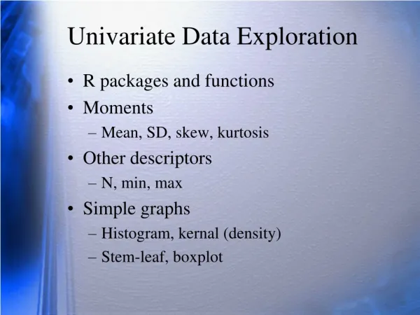
Univariate Data Exploration. R packages and functions Moments Mean, SD, skew, kurtosis Other descriptors N, min, max Simple graphs Histogram, kernal (density) Stem-leaf, boxplot. Descriptive Stats in R. You can download the R file from Canvas, Modules.

Univariate Data Exploration
E N D
Presentation Transcript
Univariate Data Exploration • R packages and functions • Moments • Mean, SD, skew, kurtosis • Other descriptors • N, min, max • Simple graphs • Histogram, kernal (density) • Stem-leaf, boxplot
Descriptive Stats in R You can download the R file from Canvas, Modules
Listing the name (e.g. Sample 1) causes the object to be printed. ‘describe’ computes the descriptive statistics
‘hist’ computes a histgram, which appears in the plot window. Click ‘Zoom’ to see it better. Hit ‘Export’ to save it to a file.
Blackmore Data • Blackmore dataset from package 'cars.' • Exercise histories of 138 girls hospitalized for eating disorders and 98 control subjects. • The data frame has 945 rows and 4 columns. • Note that there are multiple rows for each participant (but ignore for now).
Blackmore descriptives N is misleading because multiple rows per person. The SD for exercise is larger than the mean. Minimum value for exercise is zero. What do you suppose this means (also note the skew for exercise)? Group is a label for sick or control.
hist(Blackmore$age) Note how to refer to an element of an object with the $. What does this tell us about the sample?
Blackmore Exercise • hist(Blackmore$exercise)
Blackmore Exercise • exe.dens <- density(Blackmore$exercise) • plot(exe.dens)
Blackmore Exercise • boxplot(Blackmore$exercise, main='Exercise')
Why this can be a problem What a mess! Always plot your data!
Distribution Shapes • Shape of the population can be hard to infer from the sample, especially if the sample size is small. • Two different graphs showing examples of shapes. • Both sampled from N(50,2) • First is n = 100 • Second is n = 25
Shapes of Samples from Normal (n=100) Adapted from code found here: http://www.programmingr.com/content/animations-r/
Exercise • Create a ‘drive for thinness’ score and describe its distribution. • from the DavisThin dataset in car –companion for applied regression (car manual is in Canvas). Add the items to create a scale. Run descriptive stats, histogram, stem-and-leaf, boxplot.