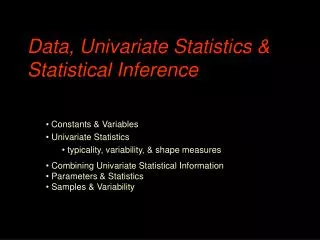
Data, Univariate Statistics & Statistical Inference

1. Data, Univariate Statistics & Statistical Inference • Constants & Variables • Univariate Statistics • typicality, variability, & shape measures • Combining Univariate Statistical Information • Parameters & Statistics • Samples & Variability

2. Measures are either Variables or Constants Constants • when all the participants in the sample have the same value on that measure/behavior Variables • when at least some of the participants in the sample have different values on that measure • either qualitative or quantitative (more later) • How do we get constants ? • Homogeneous group • everybody really has the same value • Imprecise measure • age for a group of 1st graders if measured as “# years old ” vs. “# days old” • Inadequate sample • smaller samples are more likely to have constants • non-representative (incomplete) samples more likely to have constants

3. Two Main Types of Variables Qualitative (or Categorical) • Values are mutually exclusive • Different values represent different categories / kinds • Discrete Quantitative (or Numerical) • Values are mutually exclusive • Different values represent different amounts • DiscreteorContinuous • discrete • no “partial counts” just “whole numbers” • e.g., how many siblings do you have • continuous • fractions, decimals, parts possible • must decide on level of precision • e.g., how tall are you = 6’ 5’11” 5’10.65”

4. Practice w/ Types of Variables Is each is “qual” or “quant” and if quant whether discrete or continuous ? qual quant - continuous • gender • age • major • # siblings qual quant - discreet Your Turn -- make up one of each kind… qualitative quantitative - discreet quantitative - continuous

5. Oh yeah, there’s really two more variables types … • Binary variables • qualitative variables that have two categories/values • might be “naturally occurring” -- like gender • or because we are “combining categories” (e.g., if we grouped married, separated, divorced & widowed together as “ever married” and grouped used “single” as the other category • two reasons for this… • categories are “equivalent” for the purpose of the analysis -- simplifies the analysis • too few participants in some of the samples to “trust” the data from that category • often treated as quantitative because the statistics for quantitative variables produce “sensible results”

6. The other of two other variables type … • Ordered Category Variables • multiple category variables that are formed by “sectioning” a quantitative variable • age categories of 0-10, 11-20, 21-30, 31-40 • most grading systems are like this 90-100 A, etc. • can have equal or unequal “spans” • could use age categories of 1-12 13-18 19-21 25-35 • can be binary -- “under 21” vs. “21 and older” • often treated as quantitative because the statistics for quantitative variables produce “sensible results” • but somewhat more controversy about this among measurement experts and theorists

7. Measures of Typicality (or Center) • the goal is to summarize the entire data set with a single value • stated differently … • if you had to pick one value as your “best guess” of the next participant’s score, what would it be ??? • Measures of Variability (or Spread) • the goal is to tell how much a set of scores varies or differs • stated differently … • how accurate is “best guess” likely to be ??? • Measures of Shape • primarily telling if the distribution is “symmetrical” or “skewed”

8. Measures of Typicality or Center(our “best guess”) Mode -- the “most common” score value • used with both quantitative and categorical variable Median -- “middlemost score” (1/2 of scores larger & 1/2 smaller • used with quantitative variables only • if an even number of scores, median is the average of the middlemost two scores Mean -- “balancing point of the distribution” • used with quantitative variables only • the arithmetic average of the scores (sum of scores / # of scores) Find the mode, median & mean of these scores… 1 3 3 4 5 6 Mode = 3 Median = average of 3 & 4 = 3.5 Mean = X / n = (1 + 3 + 3 + 4 + 5 + 6) / 6 = 22/6 = 3.67

9. Measures of Variability or Spread -- how good is “best guess” # categories -- used with categorical variables Range -- largest score - smallest score Standard Deviation (SD, S or std) • average difference from mean of scores in the distribution • most commonly used variability measure with quant vars • pretty nasty formula -- we’ll concentrate on using the value • “larger the std the less representative the mean” • Measures of Shape • Skewness -- summarizes the symmetry of the distribution • skewness value tells the “direction of the distribution tail” • mean & std assume distribution is symmetrical Skewness = “-” Skewness = “0” Skewness = “+”

10. Using Median & Mean to Anticipate Distribution Shape • When the distribution is symmetrical mean = median (= mode) • Mean is influenced (pulled) more than the median by the scores in the tail of a skewed distribution • So, by looking at the mean and median, you can get a quick check on the skewness of the distribution X = 56 < Med = 72 Med = 42 < X = 55 • Your turn -- what’s the skewness of each of the following distributions ? • mean = 34 median = 35 • mean = 124 median = 85 • mean = 8.2 median = 16.4 0 skewness + skewness - skewness

11. Combining Information from the Mean and Std How much does the distribution of scores vary around the mean ? • If the distribution is symmetrical • 68% of the distribution falls w/n +/- 1SD of the mean • 96% of the distribution falls w/n +/-2 SD of the mean X 68% 96% Tell me about score ranges in the following distributions ... X=20 SD=3 X=10 SD=5 68% 5-15 96% 0-20 68% 17-23 96% 14-26

12. “Beware Skewness” when combining the mean & std !!! Consider the following summary of a test • mean %-correct = 85 std = 11 • so, about 68% of the scores fall within 74% to 96% • so, about 96% of the scores fall within 63% to 107% Anyone see a problem with this ?!? 107% ???!!?? - skewed What “shape” do you think this distribution has ? Which will be larger, the mean or the median? Why think you so ?? mean < mdn • Here’s another common example… • How many times have you had stitches ? • Mean = 2.3, std = 4 68% 96% 0-7.3 0-10.3 Be sure ALL of the values in the score range are possible !!!

13. Normal Distributions and Why We Care !! • As we mentioned earlier, we can organize the sample data into a histogram, like on the right. • However, this does not provide a very efficient summary of the data. • Univariate statistics provide formulas to calculate more efficient summaries of the data (e.g., mean and standard deviation) • These stats are then the bases for other statistics that test research hypotheses (e.g., r, t, F, X²) 10 20 30 40 50 • The “catch” is that the formulas for these statistics (and all the ones you will learn this semester) depend upon the assumption that the data come from a population with a normal distribution for that variable. • Data have a normal distribution if they have a certain shape, which is represented by a really ugly formula (that we won’t worry about!!).

14. Normal distributions generally look like well-drawn versions of those shown to the right. • All normal distributions... • are symmetrical • have known proportions of the cases within certain regions of the distribution (more later) • Normal distributions differ in their … • centers (means) • spread or variability around the mean (standard deviation) Nearly all the statistics we’ll use in this class assume that the data are normally distributed. The less accurate this assumption, the greater the chance that our statistical analyses and their conclusions will be misleading.

15. Some new language … Parameter -- summary of a population characteristic Statistic -- summary of a sample characteristic Just two more … Descriptive Statistic -- calculated from sample data to describe the sample Inferential Statistic -- calculated from sample data to infer about a specific population parameter

16. Reviewing descriptive and inferential statistics … • The major difference between descriptive and inferential statistics is intent – what information you intend to get from the statistic • Descriptive statistics • obtained from the sample • used to describe characteristics of the sample • used to determine if the sample represents the target population by comparing sample statistics and population parameters • Inferential statistics • obtained from the sample • used to describe, infer, estimate, approximate characteristics of the target population • Parameters – description of population characteristics • usually aren’t obtained from the population (we can’t measure everybody) • ideally they are from repeated large samplings that produce consistent results, giving us confidence to use them as parameters

17. Another look at variability and inference ... • From those sample data we compute … • inferential mean • our best guess of the population mean • also our best guess of the score for any member of the population • inferential std • our best guess of the variability of individual scores around the population mean • the smaller the standard deviation… • the less scores vary around the mean in the population • the better the mean is as a guess of each person’s score

18. Is there any way to estimate the accuracy of our inferential mean??? Yep -- it is called the Standard Error of the Mean (SEM) and it is calculated as … std SEM = ----------------  n The SEM tells the average sampling mean sampling error -- by how much is our estimate of the population mean wrong, on the average Inferential std from sample sample size • This formula makes sense ... • the smaller the population std, the more accurate will tend to be our population mean estimate from the sample • larger samples tend to give more accurate population estimates