Download
1 / 43
430 likes | 458 Vues
This summary provides a detailed guide on how to apply the variation of parameters method to solve nth-order differential equations, covering steps from finding complementary functions to obtaining general solutions. It includes examples and key considerations for initial value problems. The method is illustrated with clear steps and explanations.

E N D
Differential Equations MTH 242 Lecture # 14 Dr. Manshoor Ahmed
Summary (Recall) • Motivation for the method of variation of parameters. • Method for first order DEs. • Method for second order DEs. • Summary of the method. • No need to add the constants. • Some examples.
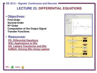
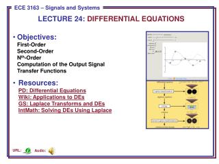
The method of variation of parameters can be applied to nth-order DE of the type. Here, we give all the steps to solve higher order DEs by variation of parameters Step 1 To find the complementary function we solve the associated homogeneous equation Step 2 Suppose that the complementary function for the equation is
Identify and find Wronskian of these linearly independent solutions. Step 4 We write the differential equation in the form and compute the determinants by replacing the column of W by the column
Step 5 Next we find the derivatives of the unknown functions through the relations Note that these derivatives can be found by solving the equations Step 6 Integrate the derivative functions computed in the step 5 to find the functions
Step 7 We write a particular solution of the given non-homogeneous equation as Step 8 The final general solution is obtained from . Note that • The first (n-1)equations in step 5 are assumptions made to simplify the first (n-1)derivatives of . The last equation in the system results from substituting the particular integral and its derivatives into the given nth order linear differential equation and then simplifying. .
Depending upon how the integrals of the derivatives of the unknown functions are found, the answer for may be different for different attempts to find for the same equation. • When asked to solve an initial value problem, we need to be sure to apply the initial conditions to the general solution and not to the complementary function alone, thinking that it is only that involves the arbitrary constants.
Example 1 Solve the differential equation by variation of parameters. Solution Step 1: The associated homogeneous equation is Auxiliary equation Therefore the complementary function is Step 2: Since
Therefore So that the Wronskian of the solutions By the elementary row operation , we have Step 3: The given differential equation is already in the required standard form
Step 4: Next we find the determinants by respectively, replacing 1st, 2nd and 3rd column of by the column
and Step 5: We compute the derivatives of the functions as: Step 6: Integrate these derivatives to find
Step 7: A particular solution of the non-homogeneous equation is Step 8: The general solution of the given differential equation is: Example 2 Solve the differential equation by variation of parameters. Solution Step 1: We find the complementary function by solving the associated homogeneous equation
Corresponding auxiliary equation is Therefore the complementary function is Step 2: Since Therefore Now we compute the Wronskian of
By the elementary row operation , we have Step 3: The given differential equation is already in the required standard form Step 4: The determinants are found by replacing the 1st, 2nd and 3rd column of by the column
Therefore and
Step 5: We compute the derivatives of the functions Step 6: We integrate these derivatives to find
Step 7: Thus, a particular solution of the non-homogeneous equation Step 8: Hence, the general solution of the given differential equation is: or or where represents .
Example 3 Solve the differential equation by variation of parameters. Solution Step 1: The associated homogeneous equation is The auxiliary equation of the homogeneous differential equation is The roots of the auxiliary equation are real and distinct. Therefore is given by
Step 2: From we find that three linearly independent solutions of the homogeneous differential equation. Thus the Wronskian of the solutions is given by By applying the row operations we obtain
Step 3: The given differential equation is already in the required standard form Step 4: Next we find the determinants by, respectively, replacing the 1st, 2nd and 3rd column of by the column Thus
and Step 5: Therefore, the derivatives of the unknown functions are given by.
Step 6: Integrate these derivatives to find Step 7: A particular solution of the non-homogeneous equation is
Step 8: The general solution of the given differential equation is:
Variation of parameters for differential equation with variable coefficients. Cauchy-Euler Equation: A linear differential equation of the form where are constants, is said to be Cauchy-Euler or equi-dimensional equation. The characteristic of this type of equation is that the degree Of the monomial coefficient is same as the order k of the differentiation :
The general solution is then Example 2: Solve .
Example 3: Solve the initial value problem .
Example 4: Solve the third order Cauchy Euler equation .
Example 5: Solve the non-homogeneous equation .
Summary • Method of variation of parameters for higher order DEs. • Higher order linear Des with variable coefficients • Method of solution for homogeneous DEs with variable coefficients. • Solution of non-homogeneous DEs with variable coefficients . • Some examples.