LECTURE 24: DIFFERENTIAL EQUATIONS
LECTURE 24: DIFFERENTIAL EQUATIONS. Objectives: First-Order Second-Order N th -Order Computation of the Output Signal Transfer Functions Resources: PD: Differential Equations Wiki: Applications to DEs GS: Laplace Transforms and DEs IntMath: Solving DEs Using Laplace. Audio:. URL:.

LECTURE 24: DIFFERENTIAL EQUATIONS
E N D
Presentation Transcript
LECTURE 24: DIFFERENTIAL EQUATIONS • Objectives:First-OrderSecond-OrderNth-OrderComputation of the Output SignalTransfer Functions • Resources:PD: Differential EquationsWiki: Applications to DEsGS: Laplace Transforms and DEsIntMath: Solving DEs Using Laplace Audio: URL:
First-Order Differential Equations • Consider a linear time-invariant system defined by: • Apply the one-sided Laplace transform: • We can now use simple algebraic manipulations to find the solution: • If the initial condition is zero, we can find the transfer function: • Why is this transfer function, which ignores the initial condition, of interest?(Hints: stability, steady-state response) • Note we can also find the frequency response of the system: • How does this relate to the frequency response found using the Fourier transform? Under what assumptions is this expression valid?
RC Circuit • The input/output differential equation: • Assume the input is a unit step function: • We can take the inverse Laplace transform to recover the output signal: • For a zero initial condition: • Observations: • How can we find the impulse response? • Implications of stability on the transient response? • What conclusions can we draw about the complete response to a sinusoid?
Second-Order Differential Equation • Consider a linear time-invariant system defined by: • Apply the Laplace transform: • If the initial conditions are zero: • Example: • What is the nature of the impulse response of this system? • How do the coefficients a0 and a1 influence the impulse response?
Nth-Order Case • Consider a linear time-invariant system defined by: • Example: • Could we have predicted the final value of the signal? • Note that all circuits involving discrete lumped components (e.g., RLC) can be solved in terms of rational transfer functions. Further, since typical inputs are impulse functions, step functions, and periodic signals, the computations for the output signal always follows the approach described above. • Transfer functions can be easily created in MATLAB using tf(num,den).
Circuit Analysis • Voltage/Current Relationships: • Series Connections (Voltage Divider):
Circuit Analysis (Cont.) • Parallel Connections (Current Divider): • Example: • Note the denominator of the transfer function did not change. Why?
RLC Circuit • Consider computation of the transfer function relating the current in the capacitor to the input voltage. • Strategy: convert the circuit to its Laplace transform representation, and use normal circuit analysis tools. • Compute the voltage across the capacitor using a voltage divider, and then compute the current through the capacitor. • Alternately, can use KVL, KVC, mesh analysis, etc. • The Laplace transform allows us to reduce circuit analysis to algebraic manipulations. • Note, however, that we can solve for both the steady state and transient responses simultaneously. • See the textbook for the details of this example.
Interconnections of Other Components • There are several useful building blocks in signal processing: integrator, differentiator, adder, subtractor and scalar multiplication. • Graphs that describe interconnections of these components are often referred to as signal flow graphs. • MATLAB includes a very nice tool, SIMULINK, to deal with such systems.
Example (Cont.) • Write equations at each node: • Subst. into the third and solve for Y(s)/X(s): • Solve for the first for Q1(s): • Subst. this into the second:
Summary • Demonstrated how to solve 1st and 2nd-order differential equations using Laplace transforms. • Generalized this to Nth-order differential equations. • Demonstrated how the Laplace transform can be used in circuit analysis. • Generalize this approach to other useful building blocks (e.g., integrator). • Next: • Generalize this approach to other block diagrams. • Work another circuit example demonstrating transient and steady-state response. • Review for exam no. 2.