Feed Sideward Und erstanding Biological Rhythms
220 likes | 370 Vues
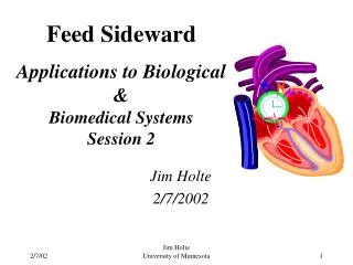
Feed Sideward Und erstanding Biological Rhythms. Jim Holte 1/15/2002. Sessions. Session 1 - Feed Sideward – Concepts and Examples, 1/15 Session 2 – Feed Sideward – Applications to Biological & Biomedical Systems, 1/31 Session 3 – Chronobiology, 2/12 Franz Hallberg and Germaine Cornalissen.

Feed Sideward Und erstanding Biological Rhythms
E N D
Presentation Transcript
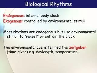
Feed SidewardUnderstandingBiological Rhythms Jim Holte 1/15/2002 Jim Holte University of Minnesota
Sessions • Session 1 - Feed Sideward – Concepts and Examples, 1/15 • Session 2 – Feed Sideward – Applications to Biological & Biomedical Systems, 1/31 • Session 3 – Chronobiology, 2/12Franz Hallberg and Germaine Cornalissen Jim Holte University of Minnesota
G In Out Σ β G In Out Σ Control G1 In Out G2 Feed Sideward TermsSimple Example • Feed Back Reinvesting dividends • Feed Foreward Setting money aside • Feed Sideward Moving money to another account Jim Holte University of Minnesota
Introduction Feed Sideward is a coupling that shifts resources from one subsystem to another • Feed Sideward #1 – feeds values of other variables into the specified variable • Feed Sideward #2 – feeds changes of parameters into the specified variable. (time varying parameters) • Feed Sideward #3 – feeds changes of topology by switch operations (switched systems) Tool for global analysis especially useful for biological systems Jim Holte University of Minnesota
Phase Space • Laws of the physical world • Ordinary differential equations • Visualization of Solutions • Understanding Jim Holte University of Minnesota
H t P P With t markers t H Phase Space The Lotka-Volterra Equations for Predator-Prey Systems H' = b*H - a*H*P P' = -d*P + c*H*P H = prey abundance, P = predator Set the parameters b = 2 growth coefficient of prey d = 1 growth coefficient of predators a = 1 rate of capture of prey per predator per unit time c = 1 rate of "conversion" of prey to predators per unit time per predator. Source: ODE Architect, Wiley, 1999 Jim Holte University of Minnesota
Phase Space The Lotka-Volterra Equations for Predator-Prey Systems H' = b*H - a*H*P P' = -d*P + c*H*P H = prey abundance, P = predator Set the parameters b = 2 growth coefficient of prey d = 1 growth coefficient of predators a = 1 rate of capture of prey per predator per unit time c = 1 rate of "conversion" of prey to predators per unit time per predator. Source: ODE Architect, Wiley, 1999 Jim Holte University of Minnesota
Coupled Oscillators Model • x and y represent the "phases“ of two oscillators. Think of x and y: • angular positions of two "particles" • moving around the unit circle • a1 = 0 • x has constant angular rate • a2 = 0 • y has constant angular rate. • Coupling when a1 or a2 non-zero Source: ODE Architect, Wiley, 1999 Jim Holte University of Minnesota
The Tortoise and the Hare x' = w1 + a1*sin(y - x) y' = w2 + a2*sin(x - y) u = (x mod(2*pi)) //Wrap around the v = (y mod(2*pi)) //unit circle phi = (x - y)mod(2*pi) Set the parameters a1 = 0.0; a2 = 0.0 w1 = pi/2; w2 = pi/3 ExampleUncoupled Oscillators Source: ODE Architect, Wiley, 1999 Jim Holte University of Minnesota
Coupled Oscillators: The Tortoise and the Hare x' = w1 + a1*sin(y - x) y' = w2 + a2*sin(x - y) u = (x mod(2*pi)) //Wrap around the v = (y mod(2*pi)) //unit circle phi = (x - y)mod(2*pi) Set the parameters a1 = 0.5; a2 = 0.5 w1 = pi/2; w2 = pi/3 ExampleCoupled Oscillators Source: ODE Architect, Wiley, 1999 Jim Holte University of Minnesota
+1 PULSE_UP STIM T1 T2 -1 PULSE_DOWN Phase Resetting FUNCTION PULSE_UP(t, T1, STIM_H) IF (t >= T1) THEN PULSE_UP = STIM_H ELSE PULSE_UP = 0 ENDIF RETURN PULSE_UP END FUNCTION STIM(t,T1,T2,STIM_L,STIM_H) STIM = PULSE_UP(t, T1, STIM_H) + PULSE_DOWN(t, T2, STIM_L) RETURN STIM END FUNCTION PULSE_DOWN(t,T2,STIM_L) IF (t <= T2) THEN PULSE_DOWN = 0 ELSE PULSE_DOWN = STIM_L ENDIF RETURN PULSE_DOWN END Jim Holte University of Minnesota
Theta' = 1 + STIM(t,T1,T2,STIM_L,STIM_H)*cos(2*Theta) T1 = 4 T2 = 4 STIM_L = -1 STIM_H = +1 Theta' = 1 + STIM(t,T1,T2,STIM_L,STIM_H)*cos(2*Theta) T1 = 4 T2 = 6 STIM_L = -1 STIM_H = +1 ExamplePhase Resetting Source: ODE Architect, Wiley, 1999 Jim Holte University of Minnesota
Oscillator Entrainment • x and y represent the "phases“ of two oscillators. • Think of x and y: • angular positions of two "particles" • moving around the unit circle • a1 = 0 • x has constant angular rate • a2 = 0 • y has constant angular rate. • Coupling when a1 & a2 non-zero • Entrainment occurs when the coupling causes • angular rate of x to • approach angular rate of y • x and y generally differ • Typical for Chronobiology • Dominant oscillator ‘entrains’ the other Source: ODE Architect, Wiley, 1999 Jim Holte University of Minnesota
Oscillator Entrainment Example x' = w1 + a1*sin(y - x) y' = w2 + a2*sin(x - y) u = (x mod(2*pi)) //Wrap around the v = (y mod(2*pi)) //unit circle phi = (x - y)mod(2*pi) Set the parameters a1 =.0775*pi; a2 =.075*pi w1 = pi/4; w2 = pi/4 - .14*pi Source: ODE Architect, Wiley, 1999 Jim Holte University of Minnesota
Singularities r' = -(r-0)*(r-1/2)*(r-1) - a*STIM(t,T1,T2,STIM_L,STIM_H) theta' = 1 x = r*cos(theta) y = r*sin(theta) T1 = 4 T2 = 6 a=0.0 STIM_L = -1 STIM_H = +1 Jim Holte University of Minnesota
Example - Singularities Run r a Commment --- --- --- --------- #1 1.25 0 approaches r=1 #2 1.0 0 stable periodic orbit #3 0.75 0 approaches r=1 #4 0.5 0 unstable periodic orbit #5 0.25 0 approaches r=0 #6 0 0 stable periodic orbit #7 0.75 0.4 starts in r=1 domain, STIM moves it to r=0 domain r' = -(r-0)*(r-1/2)*(r-1) - a*STIM(t,T1,T2,STIM_L,STIM_H) theta' = 1 x = r*cos(theta) y = r*sin(theta) T1 = 4 T2 = 6 a=0.0 STIM_L = -1 STIM_H = +1 Source: Holte & Nolley, 2002 Jim Holte University of Minnesota
G In Out Σ β G In Out Σ Control G1 In Out G2 Feed Sideward TermsSimple Example • Feed Back Reinvesting dividends • Feed Foreward Setting money aside • Feed Sideward Moving money to another account Jim Holte University of Minnesota
Feed Sideward Example The Oregonator Model for Chemical Oscillations x' = a1*(a3*y - x*y + x*(1-x)) y' = a2*(-a3*y - x*y + f*z) z' = x - z smally = y/150 a1 = 25; a3 = 0.0008; a2 = 2500; f = 1 Source: ODE Architect, Wiley, 1999 Jim Holte University of Minnesota
Summary Feed Sideward is a coupling that shifts resources from one subsystem to another • Feed Sideward #1 – feeds values of other variables into the specified variable • Feed Sideward #2 – feeds changes of parameters into the specified variable. (time varying parameters) • Feed Sideward #3 – feeds changes of topology by switch operations (switched systems) Tool for global analysis especially useful for biological systems Jim Holte University of Minnesota
Next Session • Session 1 - Feed Sideward – Concepts and Examples, 1/15 • Session 2 – Feed Sideward – Applications to Biological & Biomedical Systems, 1/31 • Session 3 – Chronobiology, 2/12Franz Hallberg and Germaine Cornelissen Jim Holte University of Minnesota
Backup Jim Holte University of Minnesota
Feed Sideward - Topics (60 min) • Session 2 (12 slides) • Applications to Biological Systems • Circadian & other Rhythms (2 slides) • Model & Simulation Result (2 slides) • Applications to Biomedical Systems • Blood Pressure Application (2 slides) • Model & Simulation Result (2 slides) • Summary (1 slide) • Segue to Chronobiology (1 slide) Session 1 (14 slides) • Background Concepts & Examples • Phase Space (1 slide) • Singularities (2 slides) * • Coupled Oscillators (2 slides) • Phase Resetting (2 slides) * • Oscillator Entrainment (1 slide) • Feed Sideward as modulation (3 slides) ** • Summary (1 slide) Jim Holte University of Minnesota