Download
1 / 66
660 likes | 738 Vues
I corsi vengono integrati e conterranno grosso modo due moduli: SB: systems biology ML: machine learning. Systems Biology. What Is It?. A branch of science that seeks to integrate different levels of information to understand how biological systems function.

E N D
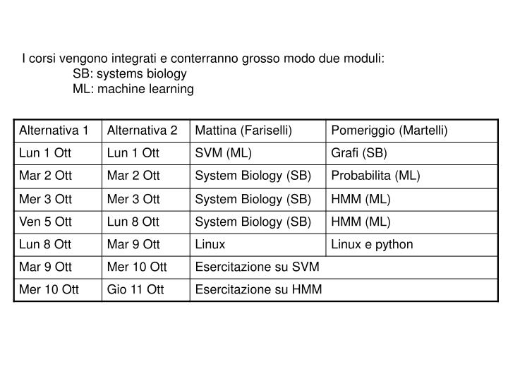
I corsi vengono integrati e conterranno grosso modo due moduli: SB: systems biology ML: machine learning
Systems Biology. What Is It? • A branch of science that seeks to integrate different levels of information to understand how biological systems function. • L. Hood: “Systems biology defines and analyses the interrelationships of all of the elements in a functioning system in order to understand how the system works.” • It is not (only) the number and properties of system elements but their relations!!
The Goal of Systems Biology: To understand the flow of mass, energy, and information in living systems. More on Systems Biology Essence of living systems is flow of mass, energy, and information in space and time. The flow occurs along specific networks • Flow of mass and energy (metabolic networks) • Flow ofinformation involving DNA (transcriptional • regulationnetworks) • Flow of information not involving DNA (signaling networks)
Networks and the Core Concepts of Systems Biology • Complexity emerges at all levels of the • hierarchy of life • System properties emerge from interactions • of components (iii) The whole is more than the sum of the parts. (iv) Applied mathematics provides approaches to modeling biological systems.
How to Describe a System As a Whole? Networks - The Language of Complex Systems
Fragment of a Social Network (Melburn, 2004) Friendship among 450 people in Canberra
A. Intra-Cellular Networks Protein interaction networks Metabolic Networks Signaling Networks Gene Regulatory Networks Composite networks Networks of Modules, Functional Networks Disease networks B. Inter-Cellular Networks Neural Networks Biological Networks C. Organ and Tissue Networks D. Ecological Networks E. Evolution Network
The Protein Interaction Network of Yeast Yeast two hybrid Uetz et al, Nature 2000
Metabolic Networks Source: ExPASy
L-A Barabasi protein-gene interactions PROTEOME protein-protein interactions METABOLISM Bio-chemical reactions Citrate Cycle GENOME miRNA regulation? _ _ _ _ _ _ _ _ _ _ _ _ _ _ _ _ _ _ _ _ _ - -
Cell Cycle Cell Polarity & Structure 7 Number of protein complexes 13 111 8 61 25 40 Number of proteins Transcription/DNA Maintenance/Chromatin Structure 77 19 15 Number of shared proteins 14 11 7 30 16 27 22 Intermediate and Energy Metabolism 187 55 740 43 221 94 33 73 83 37 103 65 11 Signaling Membrane Biogenesis & Turnover 13 20 125 20 147 53 35 321 19 41 299 49 596 75 97 Protein Synthesis and Turnover 28 692 33 419 RNA Metabolism 260 24 172 75 12 160 Protein RNA / Transport Functional Networks Yeast: 1400 proteins, 232 complexes, nine functional groups of complexes (Data A.-M. Gavin et al. (2002) Nature 415,141-147) D. Bonchev, Chemistry & Biodiversity 1(2004)312-326
What is a Network? Network is a mathematical structure composed of points connected by lines Network Theory<-> Graph Theory Network Graph Nodes Vertices (points) Links Edges (Lines) A network can be build for any functional system System vs. Parts = Networks vs. Nodes
The 7 bridges of Königsberg The question is whether it is possible to walk with a route that crosses each bridge exactly once.
The representation of Euler • In 1736 Leonhard Euler formulated the problem in terms of abstracted the case of Königsberg: • by eliminating all features except the landmasses and the bridges connecting them; • by replacing each landmass with a dot (vertex) and each bridge with a line (edge). The shape of a graph may be distorted in any way without changing the graph itself, so long as the links between nodes are unchanged. It does not matter whether the links are straight or curved, or whether one node is to the left or right of another.
The solution depends on the node degree 3 In a continuous path crossing the edges exactly once, each visited node requires an edge for entering and a different edge for exiting (except for the start and the end nodes). 3 5 3 A path crossing once each edge is called Eulerian path. It possible IF AND ONLY IF there are exactly two or zero nodes of odd degree. Since the graph corresponding to Königsberg has four nodes of odd degree, it cannot have an Eulerian path.
End 3 2 6 5 1 4 Start The solution depends on the node degree If there are two nodes of odd degree, those must be the starting and ending points of an Eulerian path.
Hamiltonian paths Find a path visiting each node exactly one Conditions of existence for Hamiltonian paths are not simple
Graph nomenclature • Graphs can be simple or multigraphs, depending on whether • the interaction between two neighboring nodes is unique or can be multiple, respectively. • A node can have or not self loops
Graph nomenclature • Networks can be undirected or directed, depending on whether • the interaction between two neighboring nodes proceeds in both • directions or in only one of them, respectively. 1 2 3 4 5 6 • The specificity of network nodes and links can be quantitatively • characterized byweights 2.5 12.7 7.3 3.3 5.4 8.1 2.5 Vertex-Weighted Edge-Weighted
Graph nomenclature trees cyclic graphs • A network can be connected (presented by a single component) or disconnected(presented by several disjoint components). connected disconnected • Networks having no cycles are termed trees. The more cycles thenetwork has, the more complex it is.
Graph nomenclature Paths Stars Cycles Complete Graphs
Vertex degree distribution (the degree of a vertex is the number of vertices connected with it via an edge) Statistical features of networks
Clustering coefficient: the average proportion of neighbours of a vertex that are themselves neighbours Node 4 Neighbours (N) 6 possible connections among the Neighbours (Nx(N-1)/2) 2 Connections among the Neighbours Statistical features of networks Clustering for the node = 2/6 Clustering coefficient: Average over all the nodes
Clustering coefficient: the average proportion of neighbours of a vertex that are themselves neighbours Statistical features of networks C=0 C=0 C=0 C=1
Given a pair of nodes, compute the shortest path between them Average shortest distance between two vertices Diameter: maximal shortest distance Statistical features of networks How many degrees of separation are they between two random people in the world, when friendship networks are considered?
How to compute the shortest path between home and work? Edge-weighted Graph The exaustive search can be too much time-consuming
The Dijkstra’s algorithm Fixed nodes NON –fixed nodes Initialization: Fix the distance between “Casa” and “Casa” equal to 0 Compute the distance between “Casa” and its neighbours Set the distance between “Casa” and its NON-neighbours equal to ∞
The Dijkstra’s algorithm Fixed nodes NON –fixed nodes Iteration (1): Search the node with the minimum distance among the NON-fixed nodes and Fix its distance, memorizing the incoming direction
4 Iteration (2): Update the distance of NON-fixed nodes, starting from the fixed distances The Dijkstra’s algorithm Fixed nodes NON –fixed nodes
The Dijkstra’s algorithm Fixed nodes NON –fixed nodes The updated distance is different from the previous one Iteration: Fix the NON-fixed nodes with minimum distance Update the distance of NON-fixed nodes, starting from the fixed distances.
The Dijkstra’s algorithm Fixed nodes NON –fixed nodes Iteration: Fix the NON-fixed nodes with minimum distance Update the distance of NON-fixed nodes, starting from the fixed distances.
The Dijkstra’s algorithm Fixed nodes NON –fixed nodes Iteration: Fix the NON-fixed nodes with minimum distance Update the distance of NON-fixed nodes, starting from the fixed distances.
The Dijkstra’s algorithm Fixed nodes NON –fixed nodes Iteration: Fix the NON-fixed nodes with minimum distance Update the distance of NON-fixed nodes, starting from the fixed distances.
The Dijkstra’s algorithm Fixed nodes NON –fixed nodes Iteration: Fix the NON-fixed nodes with minimum distance Update the distance of NON-fixed nodes, starting from the fixed distances.
The Dijkstra’s algorithm Fixed nodes NON –fixed nodes Conclusion: The label of each node represents the minimal distance from the starting node The minimal path can be reconstructed with a back-tracing procedure
Average shortest distance between two vertices Diameter: maximal shortest distance Statistical features of networks • Vertex degree distribution • Clustering coefficient
Two reference models for networks Regular network (lattice) Random network (Erdös+Renyi, 1959) Regular connections Each edge is randomly set with probability p
Two reference models for networks Comparing networks with the same number of nodes (N) and edges Poisson distribution Degree distribution Exp decay Average shortest path ≈ N ≈ log (N) high Average connectivity low
Some examples for real networks Real networks are not regular (low shortest path) Real networks are not random (high clustering)
Adding randomness in a regular network Random changes in edges OR Addition of random links
Adding randomness in a regular network (rewiring) Networks with high clustering (like regular ones) and low path length (like random ones) can be obtained: SMALL WORLD NETWORKS (Strogatz and Watts, 1999)
Small World Networks A small amount of random shortcuts can decrease the path length, still maintaining a high clustering: this model “explains” the 6-degrees of separations in human friendship network
What about the degree distribution in real networks? Both random and small world models predict an approximate Poisson distribution: most of the values are near the mean; Exponential decay when k gets higher: P(k) ≈ e-k, for large k.
What about the degree distribution in real networks? In 1999, modelling the WWW (pages: nodes; link: edges), Barabasi and Albert discover a slower than exponential decay: P(k) ≈ k-a with 2 < a < 3, for large k