Welcome Back From Spring Break
300 likes | 315 Vues
Learn about the steps for developing simulation models and how to incorporate stochastic variables. Explore the use of non-parametric distributions in financial simulation models. Review test results from previous years and understand the differences between non-parametric and parametric distributions. Gain practical knowledge on simulating random variables and applying simulation techniques in business models.

Welcome Back From Spring Break
E N D
Presentation Transcript
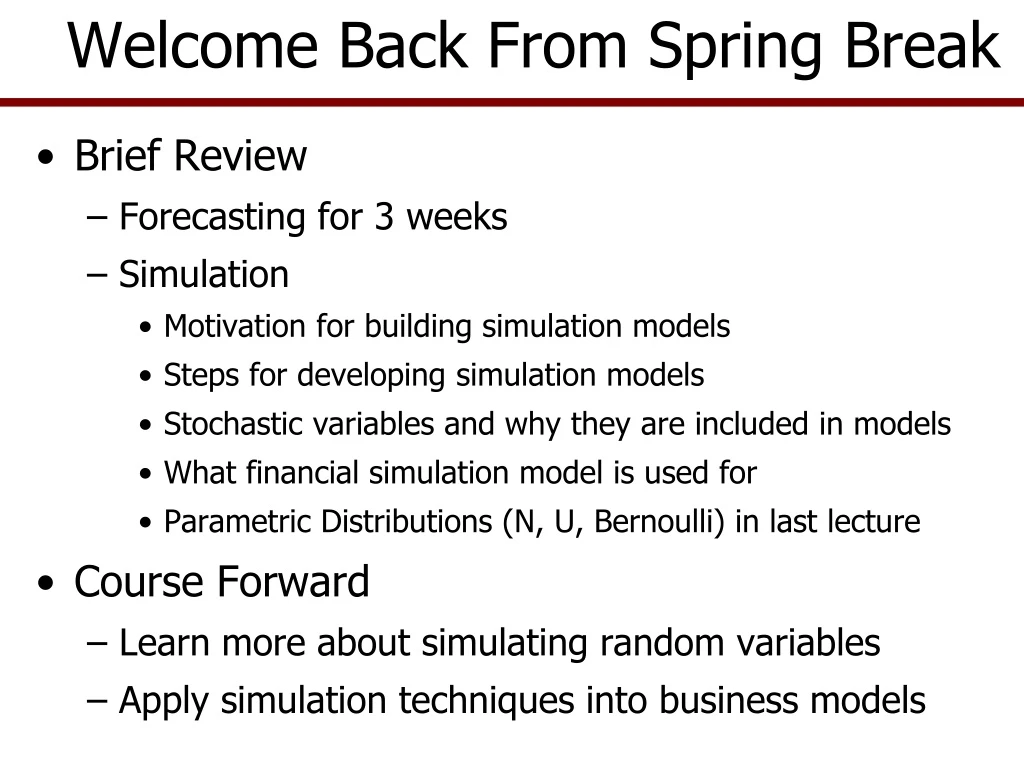
Welcome Back From Spring Break • Brief Review • Forecasting for 3 weeks • Simulation • Motivation for building simulation models • Steps for developing simulation models • Stochastic variables and why they are included in models • What financial simulation model is used for • Parametric Distributions (N, U, Bernoulli) in last lecture • Course Forward • Learn more about simulating random variables • Apply simulation techniques into business models
Test Results 2017 Mean 72.09, Std Dev 18.67, Range 26-95
Test Results 2016 Mean 81.28, Std Dev 10.38, Range 59-100
Test Results 2015 Mean 82.61, Std Dev 10.96, Range 52-99
Non-Parametric vs. Parametric Distributions • Non-Parametric Probability Distributions – not a fixed form that is parameter dependent, ex: • Discrete Uniform • Empirical • GRKS • Triangle • Parametric Distributions (covered last lecture) • Fixed form, shape dependent on parameters • Uniform, Normal, Beta, Gamma, Bernoulli
Discrete (Uniform) Empirical • Discrete Empirical distribution used where only fixed values can occur • Each value has an equal probability of being drawn • No interpolation between observed values • Examples of Discrete Empirical distributions • Discrete number of labors who show up to work • Number of live steers after a 500 mile trip • Simulating a fair die: 1, 2, 3, 4, 5, 6 • Letter grades: A, B, C, D, F
Discrete (Uniform) Empirical Distribution PDF for DE(3, 4, 6, 7) CDF for DE(3, 4, 6, 7) 1 A B C Row 1 10 2 12 .75 3 20 =DEMPIRICAL (A1:A5) function in Simetar 4 15 5 13 .5 .25 0 3 4 6 7 X 3 4 6 7 X PDF and CDF for a Discrete Uniform Distribution. - Parameters for a DE(x1, x2, x3, …, xn) based on history - Discrete Empirical means that each observed value of Xi, has an equal probability of being observed
Discrete Empirical -- Numbers • Simulate this type of random variable two ways in Simetar • Discrete empirical with equal probabilities =DEMPIRICAL(A1:A5) You can simulate DE using a USD and IF statements =EMP(A2:A6,B2:B6)
Discrete Empirical -- Alphanumeric • =RANDSORT(I1:I5) • Random shuffle 5 names-> highlight 5 cells and Type =RANDSORT(I1:I5) then press and hold Ctrl Shift Enter
Empirical Distribution • An empirical distribution is defined totally by the observations for the data, no distributional shape is assumed • Parameters to simulate an empirical distribution • Forecasted values: means (Ῡ) or forecasts (Ŷ) • Calculate percentage deviation from the mean or forecast = (Yi- Ŷi) / Ŷi • Sort the deviations from the mean (or forecast) from low to high • Assign a cumulative probability to each sorted deviate (usually assume equal probability for each data point) • Cumulative probabilities go from 0.0 to 1.0; named F(xi) or F(Si) • Assume the distribution is continuous, so interpolate between the observed points • Use the Inverse Transform formula to simulate the distribution • This requires simulation of a USD to use in the interpolation • Use Emp icon to estimate parameters in Simetar
PDF and CDF for an Empirical Dist. Probability Density Function Cumulative Distribution Function f(x) F(x) 1.0 X 0.0 max min min max X We interpolate the Dark Black line in the CDF based on the discrete CDF and use it as the approximation for a continuous distribution using the Inverse Transform method
Ỹi Stochastic Derived by linear interpolation Inverse Transform for Simulating an Empirical Distribution 1.0 F(x) Start with a random USD U(0,1) = 0.45 Interpolate the Ỹ axis using the USD value 0.0 Y1 Y2 Y6 Y3 Y4 Y5 Y7
Using the Empirical Distribution • Empirical distribution should be used if the • Random variable is continuous over its range, • You have less than 20 observations for the variable, and/or • You cannot easily estimate parameters for the true PDF • Simulate crop yields as an Empirical distribution when you have less than 20 historical values • Assume we have 10 observed yields: • Yield can be any positive value, not discrete values • We don’t have enough observations to test for normality • We know the 10 random values were observed with a probability of 1/10, or one observation each year • So F(x) goes from 0.0 to 1.0 in equal increments
Simulating Empirical Distributions • Empirical distribution is “best” simulated as percent deviations from mean or trend: percent deviates from mean = (Yt–Ῡt )/Ῡt • Parameters are: • Mean of the data is either Ῡtor Ŷt • Sorted deviations from mean or forecasted Ŷ are St = Sort [(Yt–Ῡt )/Ῡt ] using the mean as forecast or St = Sort [(Yt–Ŷt)/ Ŷt ] using trend as forecast • Probabilities for St’s, are called F(St) or F(xi) values and MUST range from 0.0 to 1.0 to use in Inverse Transform • Use the parameters to simulate random variable Ỹ: Ỹ = Ῡt * (1 + EMP(St, F(St), [USD]) )
Empirical Distribution -- No Trend • Given a random variable, Ỹ, with 11 observations • Develop the parameters if simulating variable using the mean to forecast the deterministic component: • Parameter for deterministic component is the mean or the second column • Calculate the stochastic component or ê as: êi = Yi – Ῡ • Convert residuals to fractional deviations of the forecast mean value: Devi = êi / Ῡ • Sort the Devi values from low to high (Si) and assign the probabilities of Si or F(Si) • Simulate Ỹ in two steps: Stoch Devi = EMP(Si , F(x), [USD] ) • Stoch ỸT+i = ῩT+i * (1 + Stoch Devi) • Note: Devi = (Yi- Ῡi) / Ῡirearrange terms or (Ῡ * Devi) =Yi – Ῡ so Ỹi= Ῡ + (Ῡ * Devi)
Empirical Dist. -- With Trend Parameters for EMP() if deterministic component is the trend forecast • Calculate the stochastic component or ê as: êi = Yi – Ŷi • Convert residual to fractional deviate of forecast value: Devi = êi / Ŷi • Sort the Devi values from low to high (Si) and calculate the probabilities of Si or F(Si) • Simulate Ỹ as follows: • Stoch Devi = EMP(Si, F(x), [USD] ) • ỸT+i = ŶT+i * (1 + Stoch Devi) • Derived from: Stoch Devi = (Yi - Ŷi) / Ŷi or Yi – Ŷi = (Ŷi * Stoch Devi) or Ỹi= Ŷi + (Ŷi * Stoch Devi) • ỸT+I Could have been developed from a structural or time series equation, then êi are the residuals from the regression
3 Ways to Simulate Emp Distribution • Let: Si be in B1:B10 and F(x) in A1:A10 • If Si are expressed as actual values =EMP(B1:B10) • If Si are residuals from the mean or OLS = Ῡ + EMP(B1:B10, A1:A10) • If Si are fractional deviates from mean or trendso Si = (ẽ / Ŷ) = Ŷ * (1 + EMP(B1:B10, A1:A10)) Memorize these 3 formulas. They are very important!
Simulating an EMP Distribution • Advantages of EMP Distribution • It lets the data define the shape of the distribution • Does not force an assumed distribution shape on the variable • Larger the number of observations in the sample, the closer EMP will approximate the “true” distribution • Avoids assuming a parametric distribution • Disadvantages of EMP Distribution • It has finite min and max values • It does not adhere to known probabilities and parameters • Parameters can be difficult to estimate w/o Simetar
Simulating an EMP Distribution • Advantages of specifying the Si’s as fractional deviates for forecasted values • Guarantees the “relative risk” for a random variable is the same as the historical period • Coefficient of Variation for the simulated data is constant over time CVt = (σ / Ῡt) * 100 • Allows you to use any mean (Ŷ or Ῡ) for the simulated planning horizon and simulated values have same CV as the historical period • Historical Ῡ can be 100 and the mean for the forecast period Ŷ can be 150 and the Ỹ values will have the same CV as the historical data.
GRKS Distribution • When we have insufficient historical data to estimate parameters to simulatea parametric or an Empirical distribution • Need to use expert opinion or • Use the limited data to define a distribution • Some people resort to a triangle distribution but it is really bad, as it understates the probabilities of seeing the min and max • GRKS distribution developed to simulate random variables with limited data
GRKS Distribution • Gray, Richardson, Klose and Schumann (GRKS) distribution requires three parameters • Minimum: 97.5% of observations are greater than this parameter • Middle: average or median, 50% of the observations will be less than this parameter • Maximum: 97.5% of the values are less than this parameter • Parameters are generally set based on expert opinion or limited data (less than 10 observations)
GRKS Distribution • Advantage over triangle distribution • Recognizes that there is a small probability of a value lower (or greater) than what we have observed in the past or the expert’s expectations of Min and Max • Triangle distribution is generally parameterized by asking experts what is: • the lowest value we can expect 1 year out of 10 • the highest value we can expect 1 year out of 10 • The problem is that the triangle distribution will simulate the min or max only 2% when these parameters should be observed 10% of the time, based on the experts response to the questions!
GRKS Distribution • Results of Using GRKS option in Simetar to estimate the parameters
GRKS Distribution • Simulate the GRKS using the F(x) and Sorted X values using =EMP(Sx, F(x)) • Results for the parameters are presented here
Triangle Distribution (20, 50, 100) • Note that the minimum is observed less than 1% • Note the maximum is observed less than 1% • Values <= middle observed less than 37%
GRKS Distribution • Easy to modify the GRKS distribution to represent any subjective risk or random variable. This makes the dist. very flexible. • From the Simetar Toolbar click on GRKS Distribution and fill in the menu • Edit table of deviates for Xs and F(Xs) to change the distribution shape to conform to your subjective expectations • Simulate distribution using =EMP(Si , F(x))
GRKS Distribution • The GRKS menu asks for • Minimum • Middle • Maximum • No. of intervals in Std Deviations beyond the min and max. I like 4 intervals to give more flexibility for customizing the distribution. • Always request a chart so you can see what your distribution looks like after you make changes in the X’s or Prob(x)’s
Modified GRKS Distribution GRKS in Simetar provides the F(x) and Sorted values for the distribution so they can be edited to better fit your expectations for the random variable. The bold F(x) and Sx values can be changed to develop “your own” dist. Simulate it as EMP( Sx, F(x)). I changed the Bold values below.
