Download
1 / 16
240 likes | 1k Vues
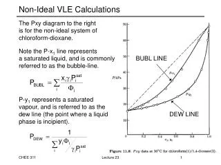
Non-Ideal VLE Calculations. The Pxy diagram to the right is for the non-ideal system of chloroform-dioxane. Note the P-x 1 line represents a saturated liquid, and is commonly BUBL LINE referred to as the bubble-line. P-y 1 represents a saturated vapour, and is referred to as the

E N D
Non-Ideal VLE Calculations • The Pxy diagram to the right • is for the non-ideal system of • chloroform-dioxane. • Note the P-x1 line represents • a saturated liquid, and is commonly BUBL LINE • referred to as the bubble-line. • P-y1 represents a saturated • vapour, and is referred to as the • dew line (the point where a liquid DEW LINE • phase is incipient). Lecture 23
Non-Ideal BUBL P Calculations • The simplest VLE calculation of the five is the bubble-point pressure calculation. • Given: T, x1, x2,…, xn Calculate P, y1, y2,…, yn • To find P, we start with a material balance on the vapour phase: • Our equilibrium relationship provides: • (14.8) • which yields the Bubble Line equation when substituted into the material balance: • or • (14.10) Lecture 23
Non-Ideal BUBL P Calculations • Non-ideal BUBL P calculations are complicated by the dependence of our coefficients on pressure and composition. • Given: T, x1, x2,…, xn Calculate P, y1, y2,…, yn • To apply the Bubble Line Equation: • requires: • ? • • • Therefore, the procedure is: • calculate Pisat, and i from the information provided • assume i=1, calculate an approximate PBUBL • use this estimate to calculate an approximate i • repeat PBUBL and i calculations until solution converges. Lecture 23
Non-Ideal Dew P Calculations • The dew point pressure of a vapour is that pressure which the mixture generates an infinitesimal amount of liquid. The basic calculation is: • Given: T, y1, y2,…, yn Calculate P, x1, x2,…, xn • To solve for P, we use a material balance on the liquid phase: • Our equilibrium relationship provides: • (14.9) • From which the Dew Line expression needed to calculate P is generated: • (14.11) Lecture 23
Non-Ideal Dew P Calculations • In trying to solve this equation, we encounter difficulties in estimating thermodynamic parameters. • Given: T, y1, y2,…, yn Calculate P, x1, x2,…, xn • ? • ? • • While the vapour pressures can be calculated, the unknown pressure is required to calculate i, and the liquid composition is needed to determine i • Assume both parameters equal one as a first estimate, calculate P and xi • Using these estimates, calculate i • Refine the estimate of xi and estimate i ((12.10ab) • Refine the estimate of P • Iterate until pressure and composition converges. Lecture 23
8. Non-Ideal Bubble and Dew T Calculations • The Txy diagram to the right • is for the non-ideal system of • ethanol(1)/toluene(2) at P =1atm. • Note the T-x1 line represents • a saturated liquid, and is commonly DEW LINE • referred to as the bubble-line. • T-y1 represents a saturated • vapour, and is referred to as the • dew line (the point where a liquid • phase is incipient). • BUBL LINE Lecture 23
Non-Ideal BUBL T Calculations • Bubble point temperature calculations are among the more complicated VLE problems: • Given: P, x1, x2,…, xn Calculate T, y1, y2,…, yn • To solve problems of this sort, we use the Bubble Line equation: • 14.10 • The difficulty in determining non-ideal bubble temperatures is in calculating the thermodynamic properties Pisat, i, and i. • Since we have no knowledge of the temperature, none of these properties can be determined before seeking an iterative solution. Lecture 23
Non-Ideal BUBL T Calculations: Procedure • 1. Estimate the BUBL T • Use Antoine’s equation to calculate the saturation temperature (Tisat) for each component at the given pressure: • Use TBUBL = xi Tisat as a starting point • 2. Using this estimated temperature and xi’s calculate • Pisat from Antoine’s equation • Activity coefficients from an Excess Gibbs Energy Model (Margule’s, Wilson’s, NRTL) • Note that these values are approximate, as we are using a crude temperature estimate. Lecture 23
Non-Ideal BUBL T Calculations: Procedure • 3. Estimate i for each component. • We now have estimates of T, Pisatand i, but no knowledge of i. • Assume that i=1 and calculate yi’s using: 14.8 • Plug P, T, and the estimates of yi’s into your fugacity coefficient expression to estimate i. • Substitute thesei estimates into 12.9 to recalculate yi and continue this procedure until the problem converges. • Step 3 provides an estimate of i that is based on the best T, Pisat, i, and xi data that is available at this stage of the calculation. • If you assume that the vapour phase is a perfect gas mixture, all i =1. Lecture 23
Non-Ideal BUBL T Calculations: Procedure • 4. Our goal is to find the temperature that satisfies our bubble point equation: • (14.10) • Our estimates of T, Pisat, i and i, are approximate since they are based on a crude temperature estimate (T = xi Tisat) • Calculate P using the Bubble Line equation (12.11) • If Pcalc < Pgiven then increase T • If Pcalc > Pgiven then decrease T • If Pcalc = Pgiven then T = TBUBL • The simplest method of finding TBUBL is a trial and error method using a spreadsheet. • Follow steps 1 to 4 to find Pcalc. • Change T and repeat steps 2, 3, and 4 until Pcalc = Pgiven Lecture 23
Non-Ideal DEW T Calculations • The dew point temperature of a vapour is that which generates an infinitesimal amount of liquid. • Given: P, y1, y2,…, yn Calculate T, x1, x2,…, xn • To solve these problems, use the Dew Line equation: • 14.11 • Once again, we haven’t sufficient information to calculate the required thermodynamic parameters. • Without T and xi’s, we cannot determine i, i or Pisat. Lecture 23
Non-Ideal DEW T Calculations: Procedure • 1. Estimate the DEW T • Using P, calculate Tisat from Antoine’s equation • Calculate T = yi Tisat as a starting point • 2. Using this temperature estimate and yi’s, calculate • Pisat from Antoine’s equation • i using the virial equation of state • Note that these values are approximate, as we are using a crude temperature estimate. Lecture 23
Non-Ideal DEW T Calculations: Procedure • 3. Estimate i, for each component • Without liquid composition data, you cannot calculate activity coefficients using excess Gibbs energy models. • A. Set i=1 • B. Calculate the Dew Pressure: • C. Calculate xi estimates from the equilibrium relationship: • D. Plug P,T, and these xi’s into your activity coefficient model to estimate i for each component. • E. Substitute these i estimates back into 12.12 and repeat B through D until the problem converges. Lecture 23
Non-Ideal DEW T Calculations: Procedure • 4. Our goal is to find the temperature that satisfies our Dew Line equation: • (14.11) • Our estimates of T, Pisat, i and i, are based on an approximate temperature (T = xi Tisat) we know is incorrect. • Calculate P using the Bubble Line equation (14.10) • If Pcalc < Pgiven then increase T • If Pcalc > Pgiven then decrease T • If Pcalc = Pgiven then T = TDew • The simplest method of finding TDew is a trial and error method using a spreadsheet. • Follow steps 1 to 4 to find Pcalc. • Change T and repeat steps 2, 3, and 4 until Pcalc = Pgiven Lecture 23
9.3 Modified Raoult’s Law • At low to moderate pressures, the vapour-liquid equilibrium equation can be simplified considerably. • Consider the vapour phase coefficient, i: • Taking the Poynting factor as one, this quantity is the ratio of two vapour phase properties: • Fugacity coefficient of species i in the mixture at T, P • Fugacity coefficient of pure species i at T, Pisat • If we assume the vapour phase is a perfect gas mixture, this ratio reduces to one, and our equilibrium expression becomes, • or 1 Lecture 23
Modified Raoult’s Law • Using this approximation of the non-ideal VLE equation simplifies phase equilibrium calculations significantly. • Bubble Points: • Setting i =1makes BUBL P calculations very straightforward. • Dew Points: Lecture 23